18.1 Introduction

In the space available, it will not be possible to cover the whole subject of motion comprehensively; instead, the aim is to provide the flavor of the subject, airing some of the principles that have proved important over the past 20 years or so. Over much of this time, optical flow has been topical, and it is appropriate to study it in fair detail, particularly, as we shall see later from some case studies on the analysis of traffic scenes, because it is being used in actual situations. Later parts of the chapter cover more modern applications of motion anaysis, including people tracking, human gait analysis, and animal tracking.

18.2 Optical Flow

When scenes contain moving objects, analysis is necessarily more complex than for scenes where everything is stationary, since temporal variations in intensity have to be taken into account. However, intuition suggests that it should be possible—even straightforward—to segment moving objects by virtue of their motion. Image differencing over successive pairs of frames should permit motion segmentation to be achieved. More careful consideration shows that things are not quite so simple, as illustrated in Fig. 18.1. The reason is that regions of constant intensity give no sign of motion, whereas edges parallel to the direction of motion also give the appearance of not moving; only edges with a component normal to the direction of motion carry information about the motion. In addition, there is some ambiguity in the direction of the velocity vector. The ambiguity arises partly because too little information is

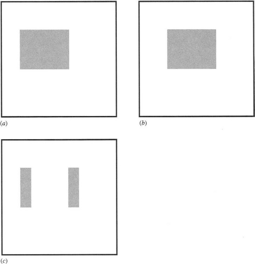
Figure 18.1 Effect of image differencing. This figure shows an object that has moved between frames (a) and (b). (c) shows the result of performing an image differencing operation. Note that the edges parallel to the direction of motion do not show up in the difference image. Also, regions of constant intensity give no sign of motion.

available within a small aperture to permit the full velocity vector to be computed (Fig. 18.2). Hence, this is called the aperture problem.

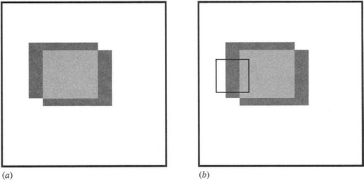
Figure 18.2 The aperture problem. This figure illustrates the aperture problem. (a) shows (dark gray) regions of motion of an object whose central uniform region (light gray) gives no sign of motion. (b) shows how little is visible in a small aperture (black border), thereby leading to ambiguity in the deduced direction of motion of the object.

Taken further, these elementary ideas lead to the notion of optical flow, wherein a local operator that is applied at all pixels in the image will lead to a motion vector field that varies smoothly over the whole image. The attraction lies in the use of a local operator, with its limited computational burden. Ideally, it would have an overhead comparable to an edge detector in

a normal intensity image—though clearly it will have to be applied locally to pairs of images in an image sequence.

We start by considering the intensity function I(x, y, t) and expanding it in a Taylor series:

     (18.1)

where second and higher order terms have been ignored. In this formula, I_x, I_y, I_t denote respective partial derivatives with respect to x, y, and t.

We next set the local condition that the image has shifted by amount (dx, dy)intimedt, so that it is functionally identical¹ at (x + dx, y + dy, t + dt) and (x, y, t):

     (18.2)

Hence, we can deduce:

     (18.3)

Writing the local velocity v in the form:

     (18.4)

we find:

     (18.5)

I_t can be measured by subtracting pairs of images in the input sequence, whereas ∇I can be estimated by Sobel or other gradient operators. Thus, it should be possible to deduce the velocity field v(x, y) using the above equation. Unfortunately, this equation is a scalar equation and will not suffice for determining the two local components of the velocity field as we require. There is a further problem with this equation—that the velocity value will depend on the values of both I_t and ∇I, and these quantities are only estimated approximately by the respective differencing operators. In both cases significant noise will arise, which will be exacerbated by taking the ratio in order to calculate v.

Let us now return to the problem of computing the full velocity field v(x, y). All we know about v is that its components lie on the following line in (v_x, v_y)-space (Fig. 18.3):

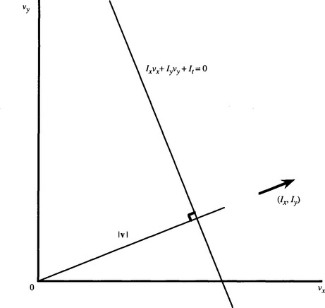
Figure 18.3 Computation of the velocity field. This graph shows the line in velocity space on which the velocity vector v must lie. The line is normal to the direction (I_x, I_y), and its distance from the origin is known to be |v| (see text).

     (18.6)

This line is normal to the direction (I_x, I_y), and has a distance from the (velocity) origin which is equal to

     (18.7)

We need to deduce the component of v along the line given by equation (18.6). However, there is no purely local means of achieving this with first derivatives of the intensity function. The accepted solution (Horn and Schunck, 1981) is to use relaxation labeling to arrive iteratively at a self-consistent solution that minimizes the global error. In principle, this approach will also minimize the noise problem indicated earlier.

In fact, problems with the method persist. Essentially, these problems arise when there are liable to be vast expanses of the image where the intensity gradient is low. In that case, only very inaccurate information is available about the velocity component parallel to ∇I, and the whole scenario becomes ill-conditioned. On the other hand, in a highly textured image, this situation should not arise, assuming that the texture has a large enough grain size to give good differential signals.

Finally, we return to the idea mentioned at the beginning of this section—that edges parallel to the direction of motion would not give useful motion information. Such edges will have edge normals normal to the direction of motion, so ∇I will be normal to v. Thus, from equation (18.5), I_t will be zero. In addition, regions of constant intensity will have ∇I .= 0, so again I_t will be zero. It is interesting and

highly useful that such a simple equation (18.5) embodies all the cases that were suggested earlier on the basis of intuition.

In the following section, we assume that the optical flow (velocity field) image has been computed satisfactorily, that is, without the disadvantages of inaccuracy or ill-conditioning. It must now be interpreted in terms of moving objects and perhaps a moving camera. We shall ignore motion of the camera by remaining within its frame of reference.

18.3 Interpretation of Optical Flow Fields

We start by considering a case where no motion is visible, and the velocity field image contains only vectors of zero length (Fig. 18.4a). Next we take a

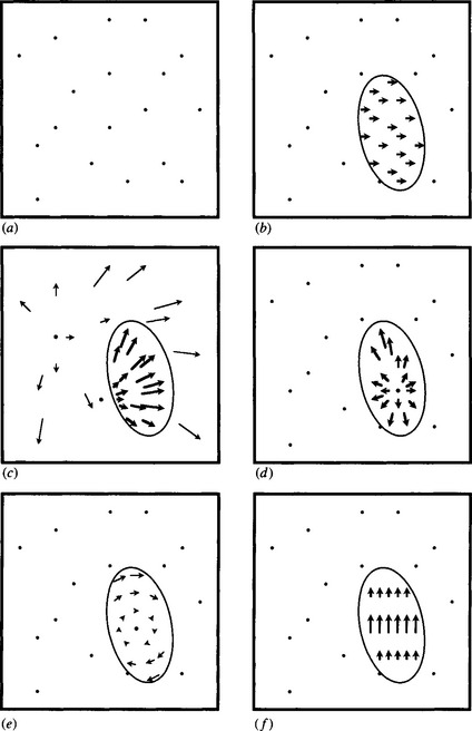
Figure 18.4 Interpretation of velocity flow fields. (a) shows a case where the object features all have zero velocity. (b) depicts a case where an object is moving to the right. (c) shows a case where the camera is moving into the scene, and the stationary object features appear to be diverging from a focus of expansion (FOE), while a single large object is moving past the camera and away from a separate FOE. In (d) an object is moving directly toward the camera which is stationary: the object’s FOE lies within its outline. In (e) an object is rotating about the line of sight to the camera, and in (f) the object is rotating about an axis perpendicular to the line of sight. In all cases, the length of the arrow indicates the magnitude of the velocity vector.

case where one object is moving toward the right, with a simple effect on the velocity field image (Fig. 18.4b). Next we consider the case where the camera is moving forward. All the stationary objects in the field of view will then appear to be diverging from a point that is called the focus of expansion (FOE)—see Fig. 18.4c. This image also shows an object that is moving rapidly past the camera and that has its own separate FOE. Figure 18.4d shows the case of an object moving directly toward the camera. Its FOE lies within its outline. Similarly, objects that are receding appear to move away from the focus of contraction. Next are objects that are stationary but that are rotating about the line of sight. For these the vector field appears as in Fig. 18.4e. A final case is also quite simple—that of an object that is stationary but rotating about an axis normal to the line of sight. If the axis is horizontal, then the features on the object will appear to be moving up or down, while paradoxically the object itself remains stationary (Fig. 18.4f)—though its outline could oscillate as it rotates.

So far, we have only dealt with cases in which pure translational or pure rotational motion is occurring. If a rotating meteor is rushing past, or a spinning cricket ball is approaching, then both types of motion will occur together. In that case, unraveling the motion will be far more complex. We shall not solve this problem here but will instead refer the reader to more specialized texts (e.g., Maybank, 1992). However, the complexity is due to the way depth (Z) creeps into the calculations. First, note that pure rotational motion with rotation about the line of sight does not depend on Z. All we have to measure is the angular velocity, and this can be done quite simply.

18.4 Using Focus of Expansion to Avoid Collision

We now take a simple case in which a focus of expansion (FOE) is located in an image, and we will show how it is possible to deduce the distance of closest approach of the camera to a fixed object of known coordinates. This type of information is valuable for guiding robot arms or robot vehicles and helping to avoid collisions.

In the notation of Chapter 16, we have the following formulas for the location of an image point (x, y, z) resulting from a world point (X, Y, Z):

     (18.8)

     (18.9)

     (18.10)

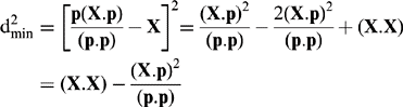
Assuming that the camera has a motion vector , fixed world points will have velocity (u, v, w) relative to the camera. Now a point (X₀, Y₀, Z₀) will after a time t appear to move to (X, Y, Z) = (X₀ + ut, Y₀ + vt, Z₀ + wt) with image coordinates:

     (18.11)

and as t → ∞ this approaches the focus of expansion F (fu/w, fv/w). This point is in the image, but the true interpretation is that the actual motion of the center of projection of the imaging system is toward the point:

     (18.12)

(This is, of course, consistent with the motion vector (u, v, w) assumed initially.) The distance moved during time t can now be modeled as:

     (18.13)

where α is a normalization constant. To calculate the distance of closest approach of the camera to the world point X = (X, Y, Z), we merely specify that the vector X_c—X be perpendicular to p (Fig. 18.5), so that:

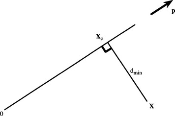
Figure 18.5 Calculation of distance of closest approach. Here the camera is moving from 0 to X_c in the direction p, not in a direct line to the object at X.dmin is the distance of closest approach.

     (18.14)

that is,

     (18.15)

     (18.16)

     (18.17)

Substituting in the equation for X_c now gives:

     (18.18)

Hence, the minimum distance of approach is given by:

     (18.19)

which is naturally zero when p is aligned along X. Avoidance of collisions requires an estimate of the size of the machine (e.g., robot or vehicle) attached to the camera and the size to be associated with the world point feature X. Finally, it should be noted that while p is obtained from the image data, X can only be deduced from the image data if the depth Z can be estimated from other information. This information should be available from time-to-adjacency analysis (see below) if the speed of the camera through space (and specifically w) is known.

18.5 Time-to-Adjacency Analysis

Next we consider the extent to which the depths of objects can be deduced from optical flow. First, note that features on the same object share the same focus of expansion, and this can help us to identify them. But how can we get information on the depths of the various features on the object from optical flow? The basic approach is to start with the coordinates of a general image point (x, y), deduce its flow velocity, and then find an equation linking the flow velocity with the depth Z.

Taking the general image point (x, y) given in equation (18.11), we find:

     (18.20)

and

     (18.21)

Hence:

     (18.22)

This result was to be expected, inasmuch as the motion of the image point has to be directly away from the focus of expansion (x_F, y_F). With no loss of generality, we now take a set of axes such that the image point considered is moving along the x-axis. Then we have:

     (18.23)

     (18.24)

Defining the distance from the focus of expansion as Δr (see Fig. 18.6), we find:

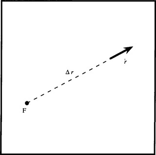
Figure 18.6 Calculation of time to adjacency. Here an object feature is moving directly away from the focus of expansion F with speed r. At the time of observation, the distance of the feature from F is Δr. These measurements permit the time to adjacency and hence also the relative depth of the feature to be calculated.

     (18.25)

     (18.26)

Equation (18.26) means that the time to adjacency, when the origin of the camera coordinate system will arrive at the object point, is the same (Z/w) when seen in real-world coordinates as when seen in image coordinates . Hence it is possible to relate the optical flow vectors for object points at different depths in the scene. This is important, for the assumption of identical values of w now allows us to determine the relative depths of object points merely from their apparent motion parameters:

     (18.27)

This is therefore the first step in the determination of structure from motion. In this context, it should be noted how the implicit assumption that the objects under observation are rigid is included—namely, that all points on the same object are characterized by identical values of w. The assumption of rigidity underlies much of the work on interpreting motion in images.

18.6 Basic Difficulties with the Optical Flow Model

When the optical flow ideas presented above are tried on real images, certain problems arise which are not apparent from the above model. First, not all edge points that should appear in the motion image are actually present. This is due to the contrast between the moving object and the background vanishing locally and limiting visibility. The situation is exactly as for edges that are produced by Sobel or other edge detection operators in nonmoving images. The contrast simply drops to a low value in certain localities, and the edge peters out. This signals that the edge model, and now the velocity flow model, is limited, and such local procedures are ad hoc and too impoverished to permit proper segmentation unaided.

Here we take the view that simple models can be useful, but they become inadequate on certain occasions and so robust methods are required to overcome the problems that then arise. Horn noted some of the problems as early as 1986. First, a smooth sphere may be rotating, but the motion will not show up in an optical flow (difference) image. If we so wish, we can regard this as a simple optical illusion, for the rotation of the sphere may well be invisible to the eye too. Second, a motionless sphere may appear to rotate as the light rotates around it. The object is simply subject to the laws of Lambertian optics, and again we may, if we wish, regard this effect as an optical illusion. (The illusion is relative to the baseline provided by the normally correct optical flow model.)

We next return to the optical flow model and see where it could be wrong or misleading. The answer is at once apparent; we stated in writing equation (18.2) that we were assuming that the image is being shifted. Yet it is not images that shift but the objects imaged within them. Thus, we ought to be considering the images of objects moving against a fixed background (or a variable background if the camera is moving). This will then permit us to see how sections of the motion edge can go from high to low contrast and back again in a rather fickle way, which we must nevertheless allow for in our algorithms. With this in mind, it should be permissible to go on using optical flow and difference imaging, even though these concepts have distinctly limited theoretical validity. (For a more thoroughgoing analysis of the underlying theory, see Faugeras, 1993.)

18.7 Stereo from Motion

An interesting aspect of camera motion is that, over time, the camera sees a succession of images that span a baseline in a similar way to binocular (stereo) images. Thus, it should be possible to obtain depth information by taking two such images and tracking object features between them. The technique is in principle more straightforward than normal stereo imaging in that feature tracking is possible, so the correspondence problem should be nonexistent. However, there is a difficulty in that the object field is viewed from almost the same direction in the succession of images, so that the full benefit of the available baseline is not obtained (Fig. 18.7). We can analyze the effect as follows.

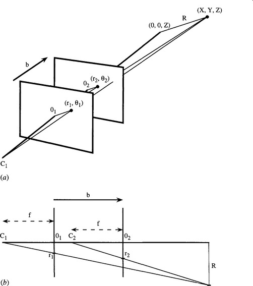
Figure 18.7 Calculation of stereo from camera motion. (a) shows how stereo imaging can result from camera motion, the vector b representing the baseline. (b) shows the simplified planar geometry required to calculate the disparity. It is assumed that the motion is directly along the optical axis of the camera.

First, in the case of camera motion, the equations for lateral displacement in the image depend not only on X but also on Y, though we can make a simplification in the theory by working with R, the radial distance of an object point from the optical axis of the camera, where:

     (18.28)

We now obtain the radial distances in the two images as:

     (18.29)

     (18.30)

so the disparity is:

     (18.31)

Writing the baseline as:

     (18.32)

and assuming that b « Z₁, Z₂, and then dropping the suffice, gives:

     (18.33)

Although this would appear to mitigate against finding Z without knowing R, we can overcome this problem by observing that:

     (18.34)

where r is approximately the mean value . Substituting for R now gives:

     (18.35)

Hence, we can deduce the depth of the object point as:

     (18.36)

This equation should be compared with equation (16.5) representing the normal stereo situation. The important point to note is that for motion stereo, the disparity depends on the radial distance r of the image point from the optical axis of the camera, whereas for normal stereo the disparity is independent of r. Asa result, motion stereo gives no depth information for points on the optical axis, and the accuracy of depth information depends on the magnitude of r.

18.8 Applications to the Monitoring of Traffic Flow

18.8.1 The System of Bascle et al.

Visual analysis of traffic flow provides an important area of 3-D and motion studies. Here we want to see how the principles outlined in the earlier chapters are brought to bear on such practical problems. In one recent study (Bascle et al., 1994) the emphasis was on tracking complex primitives in image sequences, the primitives in question being vehicles. Several aspects of the problem make the analysis easier than the general case; in particular, there is a constraint that the vehicles run on a roadway and that the motion is generally smooth. Nevertheless, the methods that have to be used to make scene interpretation reliable and robust are nontrivial and will be outlined here in some detail.

First, motion-based segmentation is used to initialize the interpretation of the sequence of scenes. The motion image is used to obtain a rough mask of the object, and then the object outline is refined by classical edge detection and linking. B-splines are used to obtain a smoother version of the outline, which is fed to a snake-based tracking algorithm.² This algorithm updates the fit of the object outline and proceeds to repeat this for each incoming image.

Snake-based segmentation, however, concentrates on isolation of the object boundary and therefore ignores motion information from the main region of the object. It is therefore more reliable to perform motion-based segmentation of the entire region bounded by the snake and to use this information to refine the description of the motion and to predict the position of the object in the next image. This means that the snake-based tracker is provided with a reliable starting point from which to estimate the position of the object in the next image. The overall process is thus to feed the output of the snake boundary estimator into a motion-based segmenter and position predictor which reinitializes the snake for the next image—so both constituent algorithms perform the operations to which they are best adapted. It is especially relevant that the snake has a good starting approximation in each frame, both to help eliminate ambiguities and to save on computation. The motion-based region segmenter operates principally by analysis of optical flow, though in practice the increments between frames are not especially small. Thus, while true derivatives are not obtained, the result is not as bedeviled by noise as it might otherwise be.

Various refinements have been incorporated into the basic procedure:

• B-splines are used to smooth the outlines obtained from the snake algorithm.

• The motion predictions are carried out using an affine motion model that works on a point-by-point basis. (The affine model is sufficiently accurate for this purpose if perspective is weak so that motion can be approximated locally by a set of linear equations.)

• A multiresolution procedure is invoked to perform a more reliable analysis of the motion parameters.

• Temporal filtering of the motion is performed over several image frames.

• The overall trajectories of the boundary points are smoothed by a Kalman filter.³

The affine motion model used in the algorithm involves six parameters:⁴

     (18.37)

This leads to an affine model of image velocities, also with six parameters:

     (18.38)

Once the motion parameters have been found from the optical flow field, it is straightforward to estimate the following snake position.

An important factor in the application of this type of algorithm is the degree of robustness it permits. In this case, both the snake algorithm and the motion-based region segmentation scheme are claimed to be rather robust to partial occlusions. Although the precise mechanism by which robustness is achieved is not clear, the abundance of available motion information for each object, the insistence on consistent motion, and the recursive application of smoothing procedures, including a Kalman filter, all help to achieve this end. However, no specific nonlinear outlier rejection process is mentioned, which could ultimately cause problems, for example, if two vehicles merged together and became separated later on. Such a situation should perhaps be treated at a higher level in order to achieve a satisfactory interpretation. Then the problem mentioned by the authors of coping with instances of total occlusion would not arise.

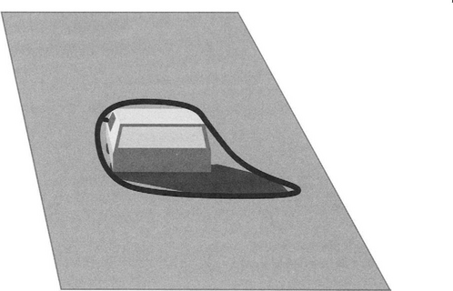
Finally, it is of interest that the initial motion segmentation scheme locates the vehicles with their shadows since these are also moving (see Fig. 18.8). Subsequent analysis seems able to eliminate the shadows and to arrive at smooth vehicle boundaries. Shadows can be an encumbrance to practical systems, and systematic rather than ad hoc procedures are ultimately needed to eliminate their effects. Similarly, the algorithm appears able to cope with cluttered backgrounds when tracking faces, though in more complex scenes this might not be possible without specific high-level guidance. In particular, snakes are liable to be confused by background structure in an image, thus, however good the starting approximation, they could diverge from appropriate answers.

Figure 18.8 Vehicles located with their shadows. In many practical situations, shadows move with the objects that cause them, and simple motion segmentation procedures produce composite objects that include the shadows. Here a snake tracker envelops the car and its shadow.

18.8.2 The System of Koller et al.

Another scheme for automatic traffic scene analysis has been described by Koller et al. (1994). This contrasts with the system described above in placing heavy reliance on high-level scene interpretation through use of belief networks. The basic system incorporates a low-level vision system employing optical flow, intensity gradient, and temporal derivatives. These provide feature extraction and lead to snake approximations to contours. Since convex polygons would be difficult to track from image to image (because the control points would

tend to move randomly), the boundaries are smoothed by closed cubic splines having 12 control points. Tracking can then be achieved using Kalman filters. The motion is again approximated by an affine model, though in this case only three parameters are used, one being a scale parameter and the other two being velocity parameters:

     (18.39)

Here the second term gives the basic velocity component of the center of a vehicle region, and the first term gives the relative velocity for other points in the region, s being the change in scale of the vehicle (s = 0 if there is no change in scale). The rationale is that vehicles are constrained to move on the roadway, and rotations will be small. In addition, motion with a component toward the camera will result in an increase in size of the object and a corresponding increase in its apparent speed of motion.

Occlusion reasoning is achieved by assuming that the vehicles are moving along the roadway and are proceeding in a definite order, so that later vehicles (when viewed from behind) may partly or wholly obscure earlier ones. This depth ordering defines the order in which vehicles are able to occlude each other, and appears to be the minimum necessary to rigorously overcome problems of occlusion.

As stated earlier, belief networks are employed in this system to distinguish between various possible interpretations of the image sequence. Belief networks are directed acyclic graphs in which the nodes represent random variables and the arcs between them represent causal connections. Each node has an associated list of the conditional probabilities of its various states corresponding to assumed states of its parents (i.e., the previous nodes on the directed network). Thus, observed states for subsets of nodes permit deductions to be made about the probabilities of the states of other nodes. Such networks are used in order to permit rigorous analysis of probabilities of different outcomes when a limited amount of knowledge is available about the system. In like manner, once various outcomes are known with certainty (e.g., a particular vehicle has passed beneath a bridge), parts of the network will become redundant and can be removed. However, before removal their influence must be “rolled up” by updating the probabilities for the remainder of the network. When applied to traffic, the belief network has to be updated in a manner appropriate to the vehicles that are currently being observed. Indeed, each vehicle will have its own belief network, which will contribute a complete description of the entire traffic scene. However, one vehicle will have some influence on other vehicles, and special note will have to be taken of stalled vehicles or those making lane changes. In addition, one vehicle slowing down will have some influence on the decisions made by drivers in following vehicles. All these factors can be encoded into the belief network and can aid in arriving at globally correct interpretations. General road and weather conditions can also be taken into account.

Further sophistication is required to enable the vision part of the system to deal with shadows, brake lights, and other signals, while it remains to be seen whether the system will be able to cope with a wide enough variety of weather conditions. Overall, the system is designed in a very similar manner to that of Bascle et al. (1994), although its use of belief networks places it in a more sophisticated and undoubtedly more robust category.

In a more recent paper (Malik et al., 1995), the same research group has found that a stereo camera scheme can be set up to use geometrical constraints in a way that improves both speed of processing and robustness. Under a number of conditions, interpretation of the disparity map is markedly simplified. The first step is to locate the ground plane (the roadway) by finding road markers such as white lines. Then the disparity map is modified to give the ground plane zero disparity. After zero ground plane disparity has been achieved, vehicles on the roadway are located trivially via their positive disparity values, reflecting their positions above the roadway. The effect is essentially one-dimensional (see Fig. 18.9). It applies only if the following conditions are valid:

1. The camera parameters are identical (e.g., identical focal lengths and image planes, optical axes parallel, etc.), differing only in a lateral baseline b.

2. The baseline vector b has a component only along the image x-axes.

3. The ground plane normal n has no component along the image x-axes.

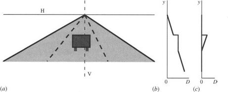
Figure 18.9 Disparity analysis of a road scene. In scene (a), the disparity D is greatest near the bottom of the image where depth Z is small, and is reduced to zero at the horizon line H. The vertical line V in the image passes up through the back of a vehicle, which is at constant depth, thereby giving constant disparity in (b). (c) shows how the disparity graph is modified when the ground plane is reduced to zero disparity by subtracting the Helmholtz shear.

In that case, there is no y-disparity, and the x-disparity on viewing the ground plane reduces to:

     (18.40)

where b is the intercamera baseline distance, h is the height of the center of projection of the camera above the ground plane, and & is the angle of declination of the optical axes below the horizontal. The conditions listed above are reasonable for practical stereo systems, and if they are valid then the disparity will have high values near the bottom of the scene, reducing to (b/h)f sin δ for vanishing points on the roadway. The next step in the calculation is to reduce the disparity of the roadway everywhere to zero by subtracting the quantity D_g from the observed disparity D. Thus, we are subtracting what has become known as the Helmholtz shear from the image. (It is a shear because the x-disparity and hence the x-values depend on y.) Here we refrain from giving a full proof of the above formula, and instead we give some insight into the situation by taking the important case δ = 0. In that case we have (cf. equation (16.4)):

     (18.41)

while from Fig. 18.10:

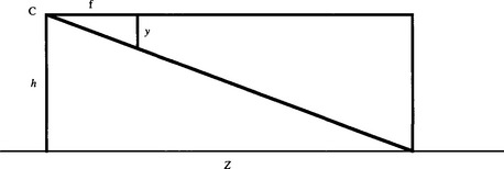
Figure 18.10 Geometry for subtracting the Helmholtz shear. Here the optical center of the camera C is a height h above the ground plane, and the optical axis of the camera is horizontal and parallel to the ground plane. The geometry of similar triangles can then be used to relate declination in the image (measured by y) to depth Z in the scene.

     (18.42)

Eliminating Z between these equations leads to:

     (18.43)

which proves the formula in that case.

Finally, whereas the subtraction of D_g from D is valid below the horizon line (where the ground plane disappears), above that level the definition of D_g is open to question. Equation (18.40) could provide an invalid extrapolation above the horizon line (would zero perhaps be a more appropriate value?). Assuming that equation (18.40) remains valid and that D_g is negative above the horizon line, then we will be subtracting a negative quantity from the observed disparity. Thus, the deduced disparity will increase with height. By way of example, take two telegraph poles equidistant from the camera and placed on either side of the roadway. Their disparity will now increase with height, and as a result they will appear to have a separation that also increases with height. It turns out that this was the form of optical illusion discovered by von Helmholtz (1925), which led him to the hypothesis that a shear (equation (18.40)) is active within the human visual system. In the context of machine vision, it is clearly a construction that has a degree of usefulness, but also carries important warnings about the possibility of making misleading measurements from the resulting sheared images. The situation arises even for the backs of vehicles seen below the horizon line (see Fig. 18.9c).

18.9 People Tracking

Visual surveillance is a long-standing area of computer vision, and one of its main early uses was to obtain information on military activities—whether from high-flying aircraft or from satellites. However, with the advent of ever cheaper video cameras, it next became widely used for monitoring road traffic, and most recently it has become ubiquitous for monitoring pedestrians. In fact, its application has actually become much wider than this, the aim being to locate criminals or people acting suspiciously—for example, those wandering around car-parks with the potential purpose of theft. By far the majority of visual surveillance cameras are connected to video recorders and gather miles of videotape, most of which will never be looked at—although following criminal or other activity, hours of videotape may be scanned for relevant events. Further cameras will be attached to closed circuit television monitors where human operators may be able to extract some fraction of the events displayed, though human attentiveness and reliability when overseeing a dozen or so screens will not be high. It would be far better if video cameras could be connected to automatic computer vision monitoring systems, which would at the minimum call human operators’ attention to potential hazards or misdemeanors. Even if this were not carried out in real time in specific applications, it would be useful if it could be achieved at high speed with selected videotapes. This could save huge amounts of police time in locating and identifying perpetrators of crime.

Surveillance can cover other useful activities, including riot control, monitoring of crowds at sports events, checking for overcrowding in underground stations, and generally helping in matters of safety as well as crime. To some extent, human privacy must be sacrificed when surveillance is called into play, and a tradeoff between privacy and security then becomes necessary. Suffice it to say that many would consider a small loss of privacy a welcome price to pay to achieve increased security.

Many difficulties must be overcome before the “people-tracking” aspects of surveillance are fully solved. First, in comparison to cars, people are articulated objects that change shape markedly as they move. That their motion is often largely periodic can help visual analysis, though the irregularities in human motion may be considerable, especially if obstacles have to be avoided. Second, human motions are partly self-occluding, one leg regularly disappearing behind another, while arms can similarly disappear from view. Third, people vary in size and apparent shape, having a variety of clothes that can disguise their outlines. Fourth, when pedestrians are observed on a pavement, or on the underground, it is possible to lose track when one person passes behind another, as the two images coalesce before reemerging from the combined object shape.

It could be said that all these problems have been solved, but many of the algorithms that have been applied to these tasks have limited intelligence. Indeed, some employ rather simplified algorithms, as the need to operate continuously in real time frequently overrides the need for absolute accuracy. In any case, given the visual data that the computer actually receives, it is doubtful whether a human operator could always guarantee getting correct answers. For example, on occasions humans turn around in their tracks because they have forgotten something, thereby causing confusion when trying to track every person in a complex scene.

Further complexities can be caused by varying lighting, fixed shadows from buildings, moving shadows from clouds or vehicles, and so on.

18.9.1 Some Basic Techniques

The majority of people trackers use a motion detector to start the process of tracking. In principle, a model of the background can be taken with no people present, and then regions of interest (ROIs) can be formed around any substantial regions where movement is detected. However, such an approach will be error-prone, because changes in lighting or new placards, and so on, will appear to be people, and second because after people have criss-crossed the scene many times, error propagation will ensure many erroneous pixel classifications. Instead, it is usual to update the background model either by taking a temporal median of the scene (i.e., updating each pixel independently by using a running temporal median of the image sequence), or by some equivalent procedure that ignores outliers caused by temporary passage of moving objects, including people. Then, image differencing relative to the background model can yield quite reliable ROIs for the various people in the scene. Typically, these ROIs are rectangular in shape and can conveniently be moved with the people around the scene (Fig. 18.11). However, when people’s paths cross, complications occur, and the ROIs tend to merge. Such problems have to be overcome by additional region-splitting procedures, often aided by Kalman filters that can help predict the motion over the merger period, thereby efficiently arriving at optimal tracking solutions. Since this approach is somewhat ad hoc, the emphasis has moved to more exact modeling of human shapes, using the ROIs merely as helpful approximations.

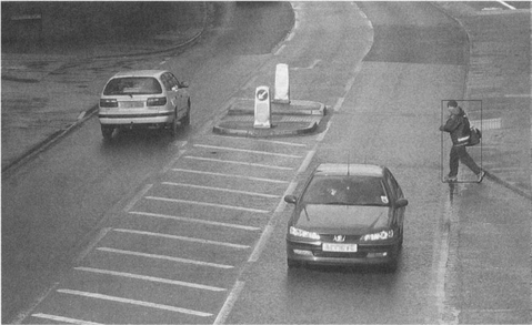
Figure 18.11 Example of a rectangular region of interest around a pedestrian. When outlined on a picture, the ROI is frequently called a bounding box.

The Leeds people tracker (Baumberg and Hogg, 1995) learned a large number of walking pedestrian shapes and represented them as a set of cubic B-spline contours with N control points. These shapes were then analyzed using principal components analysis (Chapter 24) to find the possible “modes of variation” (eigenshapes) for the training data. The principal mode of variation is depicted by the extremes shown in Fig. 18.12. Although to the human eye these shapes do not match the average pedestrian well, they represent a substantial improvement over the basic rectangular ROI concept. In addition, they are well parametrized, in such a way that tracking is facilitated—and of course spatiotemporal shape development can be matched with the shapes that appear within the scene.

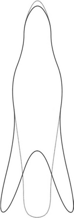
Figure 18.12 Eigenshapes of pedestrians. The two traces show typical extremes of the principal mode of variation of pedestrian shapes, as generated by PCA and characterized by cubic B-splines. Though constrained, this parametrization is actually very useful and far more powerful than the standard rectangular ROI representation (see text).

The Siebel and Maybank (2002) people tracker incorporates the Leeds people tracker but also includes a head detector. The overall system contains a motion

detector (using a temporal median filter), a region tracker, a head detector, and an active shape tracker. Note that the temporal median approach leads to static objects eventually being incorporated into the background—a process that must not be undertaken too quickly, for it could even lead to creation of a negative object when a stationary pedestrian decides to move on. Siebel and Maybank took particular care to avoid this type of problem by keeping alert to objects for some time after they had become static. They also devoted considerable effort to developing a tracking history for the whole system. This permitted the four main modules, including the region tracker and the active shape tracker, to have access to each other in case any individual module lost data or lost track. This allowed the whole system to make up for deficiencies in any of its modules and thus improved overall tracking performance. The overall system employs hypothesis refinement, generating and running several track hypotheses per tracked person. Normally only one track is retained, but if occlusions or dropped frames occur, more are retained on a temporary basis.

The overall system was much more reliable than the active shape tracker at its core, (1) because it did not lose track of a person so easily, (2) because it incorporated more features into the region tracker, and (3) because its history tracking facility meant that it could regain some tracks previously lost.

In summary, as Siebel and Maybank (2002) have observed, there are three main categories of people tracking, of increasing complexity: (1) region- or blob-based tracking, using 2-D segmentation; (2) 2-D appearance modeling of human beings; and (3) full 3-D modeling of human beings. Because the

third category tends to run too slowly for practical cost-effective real-time applications, Siebel and Maybank concentrated on the second approach.

18.10 Human Gait Analysis

For well over a decade human motion has been studied using conventional cinematography. Often the aim of this work has been to analyze human movements in the context of various sports—in particular tracking the swing of a golf club and thus aiding the player in improving his game. To make the actions clearer, stroboscopic analysis coupled with bright markers judiciously placed on the body have been employed and have resulted in highly effective action displays. In the 1990s, machine vision was applied to the same task. At this point, the studies became much more serious, and there was greater focus on accuracy because of a widening of the area of application not only to other sports but also to medical diagnosis and to animation for modern types of films containing artificial sequences.

Because a high degree of accuracy is needed for many of these purposes—not the least of which is measuring limps or other imperfections of human gait—analysis of the motion of the whole human body in normally lit scenes proved insufficient, and body markers remained important. Typically, two body markers are needed per limb, so that the 3-D orientation of each limb will be deducible.

Some work has been done to analyze human motions using single cameras, but the majority of the work employs two or more cameras. Multiple cameras are valuable because of the regular occlusion that occurs when one limb passes behind another, or behind the trunk.

To proceed with the analysis, a kinematic model of the human body is required. In general, such models assume that limbs are rigid links between a limited number of ball and socket joints, which can be approximated as point junctions between stick limbs. One such model (Ringer and Lazenby, 2000) employs two rotation parameters for the location where the hips join the backbone and three for the joint where the thigh bone joins the hips, plus one for the knee and another for the ankle. Thus, there are seven joint parameters for in each leg, two of these being common (at the backbone). This leads to a total of 12 parameters covering leg movements (Fig. 18.13). While it is part of the nature of the skeleton that the joints are basically rotational, there is some slack in the system, especially in the shoulders, while the backbone, which is compressed when upright, extends slightly when lying down or when hanging. In addition, the knee has some lateral freedom. A full analysis will be highly complex, though achieving it will be worthwhile for measuring mobility for medical diagnostic purposes. Finally, the whole situation is made more complex by constraints such as the inability of the knee to extend the lower leg too far forward.

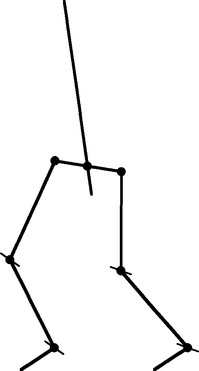
Figure 18.13 Stick skeleton model of the lower human body. This model takes the main joints on the skeleton as being universal ball-and-socket joints, which can be approximated by point junctions—albeit with additional constraints on the possible motions (see text). Here a thin line through a joint indicates the single rotational axis of that joint.

Once a kinematic model has been established, tracking can be undertaken. It is relatively straightforward to identify the markers on the body with reasonable accuracy—though quite often one may be missed because of occlusion or because of poor lighting or the effects of noise. The next problem is to distinguish one marker from another and to label them. Considering the huge number of combinations of labels that are possible in the worst case scenario, and the frequency with which occlusions of parts of the farside leg or arm are bound to take place, special association algorithms are required for the purpose. These algorithms include particularly the Kalman filter, which is able to help predict how unseen markers will move until they come back into view. Such methods can be improved by including acceleration parameters as well as position and velocity parameters in the model (Dockstader and Tekalp, 2002). The model of Dockstader and Tekalp (2002) is not merely theoretically deduced: it has to be trained, typically on sequences of 2500 images each separated by 1/30 sec. Even so, the stick model of each human subject has to be initialized manually. A large amount of training is necessary to overcome the slight inaccuracies of measurement and to build up the statistics sufficiently for practical application when testing. Errors are greatest when measuring hand and arm movements because of the frequent occlusions to which they are subject.

Overall, articulated motion analysis involves complex processing and a lot of training data. It is a key area of computer vision, and the subject is evolving rapidly. It has already reached the stage of producing useful output, but accuracy will improve over the next few years. This will set the scene for practical medical monitoring and diagnosis, completely natural animation, detailed help with sports activities at costs that can be afforded by all, not to mention recognition of criminals by their characteristic gaits. Certain requirements—such as multiple cameras—will probably remain, but there will doubtless be a trend to markerless monitoring and minimal training on specific individuals (though there will still need to be bulk training on a sizable number of individuals). This is a fascinating and highly appropriate application of machine vision, and current progress indicates that it will essentially be solved within a decade.⁷

18.11 Model-based Tracking of Animals—A Case Study

This case study is concerned with animal husbandry—the care of farm animals. Good stockmen notice many aspects of animal behavior, and learn to respond to them. Fighting, bullying, tail biting activity, resting behavior, and posture are useful indicators of states of health, potential lameness, or heat stress, while group behavior may indicate the presence of predators or human intruders. In addition, feeding behavior is all important, as is the incidence of animals giving birth or breaking away from the confinement of the pen. In all these aspects, automatic observation of animals by computer vision systems is potentially useful.

Some animals such as pigs and sheep are lighter than their usual backgrounds of soil and grass, and thus they can in principle be located by thresholding. However, the backgrounds may be cluttered with other objects such as fences, pen walls, drinking troughs, and so on—all of which will complicate interpretation. Whatever the situation on factory conveyors, straightforward thresholding is unlikely to work well in normal outdoor and indoor farm scenes.

McFarlane and Schofield (1995) tackled this problem by image differencing. While differencing between adjacent frames is useful only if specific motion is occurring, far better performance may be achieved if the current frame is differenced against a carefully prepared background image. Employing such an image might seem to be a panacea, but this is not so, as the ambient lighting will vary throughout the day, and care must be taken to ensure that no animals are present when a background image is being taken. McFarlane and Schofield used a background image obtained by finding the median intensity at each pixel for a whole range of images taken over a fair period, in an effort to overcome this problem. Intelligent applications of this procedure were instituted to mask out regions where piglets were known to be resting. In such applications, medians are more effective than mean values, for they robustly eliminate outlier values rather than averaging them in.

The McFarlane and Schofield algorithm modeled piglets as simple ellipses and had fair success with their approach. However, next we examine the more rigorous modeling approach adopted by Marchant and Onyango (1995), and developed further by Onyango and Marchant (1996) and Tillett et al. (1997). These workers aimed to track the movements of pigs within a pen by viewing them from overhead under not too uniform lighting conditions. The main aim of the work at this early stage was tracking the animals, though, as indicated earlier, it was intended to lead on to behavioral analysis in later work. To find the animals, some form of template matching is required. Shape matching is an attractive concept, but with live animals such as pigs, the shapes are highly variable. Specifically, animals that are standing up or walking around will bend from side to side and may also bend their necks sideways or up and down as they feed. It is insufficient to use a small number of template masks to match the shapes, for there is an infinity of shapes related by various values of the shape parameters mentioned. These parameters are in addition to the obvious ones of position, orientation, and size.

Careful trials show that matching with all these parameters is insufficient, for the model is quite likely to be shifted laterally by variations in illumination. If one side of a pig is closer to the source of illumination, it will be brighter, and hence the final template used for matching will also shift in that direction. The resulting fit could be so poor that any reasonable goodness of fit criterion may deny the presence of a pig. Possible variations in lighting therefore have to be taken fully into account in fitting the animal’s intensity profile.

A full-blooded approach involves principal components analysis (PCA). The deviation in position and intensity between the training objects and the model at a series of carefully chosen points is fed to a PCA system. The highest energy eigenvalues indicate the main modes of variation to be expected. Then any specific test example is fitted to the model, and amplitudes for each of these modes of variation are extracted, together with an overall parameter representing the goodness of fit. Unfortunately, this rigorous approach is highly computation intensive, because of the large number of free parameters. In addition, the position and intensity parameters are disparate measures that require the use of totally different and somewhat arbitrary scale factors to help the schema work. Some means is therefore required for decoupling the position and intensity information. Decoupling is achieved by performing two independent principal components analyses in sequence—first on the position coordinates and then on the intensity values.

When this procedure was carried out, three significant shape parameters were found, the first being lateral bending of the pig’s back, accounting for 78% of the variance from the mean; and the second being nodding of the pig’s head, which, because it corresponded to only ~20% of the total variance, was ignored in later analysis. In addition, the gray-level distribution model had three modes of variation, amounting to a total of 77% of the intensity variance. The first two modes corresponded to (1) a general amplitude variation in which the distribution is symmetrical about the backbone, and (2) a more complex variation in which the intensity distribution is laterally shifted relative to the backbone. (This clearly arises largely from lateral illumination of the animal.) See Fig. 18.14.

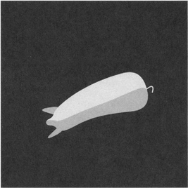
Figure 18.14 Effect of one mode of intensity variation found by PCA. This mode clearly arises from lateral illumination of the pig.

Although principal components analyses yield the important modes of variation in shape and intensity, in any given case the animal’s profile has still to be fitted using the requisite number of parameters—one for shape and two for intensity. The Simplex algorithm (Press et al., 1992) has been found effective for this purpose. The objective function to be minimized to optimize the fit takes account of (1) the average difference in intensity between the rendered (gray-level)

model and the image over the region of the model; and (2) the negative of the local intensity gradient in the image normal to the model boundary averaged along the model boundary. (The local intensity gradient will be a maximum right around the animal if this is correctly outlined by the model.)

One crucial factor has been skirted over in the preceding discussion: that the positioning and alignment of the model to the animal must be highly accurate (Cootes et al., 1992). This applies both for the initial PCA and later when fitting individual animals to the model is in progress. Here we concentrate on the PCA task. It should always be borne in mind when using PCA that the PCA is a method of characterizing deviations. This means that the deviations must already be minimized by referring all variations to the mean of the distribution. Thus, when setting up the data, it is very important to bring all objects to a common position, orientation, and scale before attempting PCA. In the present context, the PCA relates to shape analysis, and it is assumed that prior normalizations of position, orientation, and scale have already been carried out. (Note that in more general cases scaling may be included within PCA if required. However, PCA is a computation-intensive task, and it is best to encumber it as little as possible with unnecessary parameters.)

Overall, the achievements outlined here are notable, particularly in the effective method for decoupling shape and intensity analysis. In addition, the work holds significant promise for application in animal husbandry, demonstrating that animal monitoring and ultimately behavioral analysis should, in the foreseeable future, be attainable with the aid of image processing.

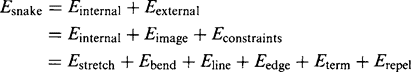
18.12 Snakes

There have been more than a dozen mentions of snakes (also known as deformable contours or active contour models) in this chapter, and it is left to this section to explain what they are and how they are computed.

The basic concept of snakes involves obtaining a complete and accurate outline of an object that may be ill-defined in places, whether through lack of contrast or noise or fuzzy edges. A starting approximation is made either by instituting a large contour that may be shrunk to size, or a small contour that may be expanded suitably, until its shape matches that of the object. In principle, the initial boundary can be rather arbitrary, whether mostly outside or within the object in question. Then its shape is made to evolve subject to an energy minimization process. On the one hand, it is desired to minimize the external energy corresponding to imperfections in the degree of fit; on the other hand, it is desired to minimize the internal energy, so that the shape of the snake does not become unnecessarily intricate, for example, taking on any of the characteristics of image noise. There are also model constraints that are represented in the formulation as contributions to the external energy. Typical of such constraints is that of preventing the snake from moving into prohibited regions, such as beyond the image boundary, or, for a moving vehicle, off the region of the road.

The snake’s internal energy includes elastic energy, which might be needed to extend or compress it, and bending energy. If no bending energy terms were included, sharp corners and spikes in the snake would be free to occur with no restriction. Similarly, if no elastic energy terms were included, the snake would be permitted to grow or shrink without penalty.

The image data are normally taken to interact with the snake via three main types of image features: lines, edges, and terminations (the last-named can be line terminations or corners). Various weights can be given to these features according to the behavior required of the snake. For example, it might be required to hug edges and go around corners, and only to follow lines in the absence of edges. So the line weights would be made much lower than the edge and corner weights.

These considerations lead to the following breakdown of the snake energy:

     (18.45)

The energies are written down in terms of small changes in position x(s) = (x(s), y(s)) of each point on the snake, the parameter s being the arc length distance along the snake boundary. Thus we have:

     (18.46)

and

     (18.47)

where the suffices s, ss imply first- and second-order differentiation, respectively. Similarly, E_edge is calculated in terms of the intensity gradient magnitude |gradI|, leading to:

     (18.48)

where wedge is the edge-weighting factor.

The overall snake energy is obtained by summing the energies for all positions on the snake; a set of simultaneous differential equations is then set up to minimize the total energy. Space prevents a full discussion of this process here. Suffice it to say that the equations cannot be solved analytically, and recourse has to be made to iterative numerical solution, during which the shape of the snake evolves from some high-energy initialization state to the final low-energy equilibrium state, defining the contour of interest in the image.

In the general case, several possible complications need to be tackled:

Procedural problems also exist. The intrinsic snake concept is that of well-behaved differentiability. However, lines, edges, and terminations are usually highly localized, so there is no means by which a snake even a few pixels away could be expected to learn about them and hence to move toward them. In these circumstances the snake would “thrash around” and would fail to systematically zone in on a contour representing a global minimum of energy. To overcome this problem, smoothing of the image is required, so that edges can communicate with the snake some distance away, and the smoothing must gradually be reduced as the snake nears its target position. Ultimately, the problem is that the algorithm has no high-level appreciation of the overall situation, but merely reacts to a conglomerate of local pieces of information in the image. This makes segmentation using snakes somewhat risky despite the intuitive attractiveness of the concept.

In spite of these potential problems, a valuable feature of the snake concept is that, if set up correctly, the snake can be rendered insensitive to minor discontinuities in a boundary. This is important, for this makes it capable of negotiating practical situations such as fuzzy or low-contrast edges, or places where small artifacts get in the way. (This may happen with resistor leads, for example.) This capability is possible because the snake energy is set up globally—quite unlike the situation for boundary tracking where error propagation can cause wild deviations from the desired path. The reader is referred to the abundant literature on the subject (e.g., see Section 18.15) not only to clarify the basic theory (Kass and Witkin, 1987; Kass et al., 1988) but also to find how it may be made to work well in real situations.

18.13 The Kalman Filter

When tracking moving objects, it is desirable to be able to predict where they will be in future frames, for this will make maximum use of preexisting information and permit the least amount of search in the subsequent frames. It will also serve to offset the problems of temporary occlusion, such as when one vehicle passes behind another, when one person passes behind another, or even when one limb of a person passes behind another. (There are also many military needs for tracking prediction, and others on the sports field.) The obvious equations to employ for this purpose involve sequentially updating the position and the velocity of points on the object being tracked:

     (18.49)

     (18.50)

assuming for convenience a unit time interval between each pair of samples.

This approach is too crude to yield the best results. First, it is necessary to make three quantities explicit: (1) the raw measurements (e.g., x), (2) the best estimates of the values of the corresponding variables before observation (denoted by -), and (3) the best estimates of these same model parameters following observation (denoted by ⁺). In addition, it is necessary to include explicit noise terms, so that rigorous optimization procedures can be derived for making the best estimates.

In the particular case outlined above, the velocity—and possible variations on it, which we shall ignore here for simplicity—constitutes a best estimate model parameter. We include position measurement noise by the parameter u and velocity (model) estimation noise by the parameter w. The above equations now become:

     (18.51)

     (18.52)

In the case where the velocity is constant and the noise is Gaussian, we can spot the optimum solutions to this problem:

     (18.53)

     (18.54)

these being called the prediction equations, and

     (18.55)

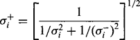     (18.56)

these being called the correction equations.⁸ (In these equations, σ^± are the standard deviations for the respective model estimates x^±, and a is the standard deviation for the raw measurements x.)

These equations show how repeated measurements improve the estimate of the position parameter and the error upon it at each iteration. Notice the particularly important feature—that the noise is being modeled as well as the position itself. This permits all positions earlier than i—1 to be forgotten. The fact that there were many such positions, whose values can all be averaged to improve the accuracy of the latest estimate, is of course rolled up into the values of x_i^— and σ_i^—, and eventually into the values for x_i⁺ and σ_i⁺.

The next problem is how to generalize this result, both to multiple variables and to possibly varying velocity and acceleration. The widely used Kalman filter performs the required function by continuing with a linear approximation and by employing a state vector comprising position, velocity, and acceleration (or other relevant parameters), all in one state vector s. This constitutes the dynamic model. The raw measurements x have to be considered separately.

In the general case, the state vector is not updated simply by writing:

     (18.57)

but requires a fuller exposition because ofthe interdependence of position, velocity, and acceleration. Hence we have:⁹

     (18.58)

Similarly, the standard deviations σ_i, σ_i^— in equations (18.54)-(18.56) (or rather, the corresponding variances) have to be replaced by the covariance matrices Σ_i, Σ_i^±,and the equations become significantly more complicated. We will not go into the calculations fully here because they are nontrivial and would need several pages to iterate. Suffice it to say that the aim is to produce an optimum linear filter by a least-squares calculation (see, for example, Maybeck, 1979).

Overall, the Kalman filter is the optimal estimator for a linear system for which the noise is zero mean, white, and Gaussian, though it will often provide good estimates even if the noise is not Gaussian.

Finally, it will be noticed that the Kalman filter itself works by averaging processes that will give erroneous results if any outliers are present. This will certainly occur in most motion applications. Thus, there is a need to test each prediction to determine whether it is too far away from reality. If this is the case, the object in question will not likely have become partially or fully occluded. A simple option is to assume that the object continues in the same motion (albeit with a larger uncertainty as time goes on) and to wait for it to emerge from behind another object. At the very least, it is prudent to keep a number of such possibilities alive for some time, but the extent of this will naturally vary from situation to situation and from application to application.

18.14 Concluding Remarks

Early in this chapter we described the formation of optical flow fields and showed how a moving object or a moving camera leads to a focus of expansion. In the case of moving objects, the focus of expansion can be used to decide whether a collision will occur. In addition, analysis of the motion taking account of the position of the focus of expansion led to the possibility of determining structure from motion. Specifically, the calculation can be achieved via time-to-adjacency analysis, which yields the relative depth in terms of the motion parameters measurable directly from the image. We then went on to demonstrate some basic difficulties with the optical flow model, which arise since the motion

edge can have a wide range of contrast values, making it difficult to measure motion accurately. In practice, larger time intervals may have to be employed to increase the motion signal. Otherwise, feature-based processing related to that of Chapter 15 can be used. Corners are the most widely used feature for this purpose because of their ubiquity and because they are highly localized in 3-D. Space prevents details of this approach from being described here: details may be found in Barnard and Thompson (1980), Scott (1988), Shah and Jain (1984), and Ullman (1979).

Section 18.8 presented a study of two vision systems that have recently been developed with the purpose of monitoring traffic flow. These systems are studied here in order to show the extent to which optical flow ideas can be applied in real situations and to determine what other techniques have to be used to build complete vision systems for this type of application. Interestingly, both systems made use of optical flow, snake approximation to boundary contours, affine models of the displacements and velocity flows, and Kalman filters for motion prediction—confirming the value of all these techniques. On the other hand, the Koller system also employed belief networks for monitoring the whole process and making decisions about occlusions and other relevant factors. In addition, the later version of the Koller system (Malik, 1995) used binocular vision to obtain a disparity map and then applied a Helmholtz shear to reduce the ground plane to zero disparity so that vehicles could be tracked robustly in crowded road scenes. Ground plane location was also a factor in the design of the system.

Later parts of the chapter covered more modern applications of motion analysis, including people tracking, human gait analysis, and animal tracking. These studies reflect the urgency with which machine vision and motion analysis are being pursued for real applications. In particular, studies of human motion reflect medical and film production interests, which can realistically be undertaken on modern high-speed computer platforms.

Further work related to motion will be covered in Chapter 20 after perspective invariants have been dealt with (in Chapter 19), for this will permit progress on certain aspects of the subject to be made more easily.

18.15 Bibliographical and Historical Notes

Optical flow has been investigated by many workers over many years: see, for example, Horn and Schunck (1981) and Heikkonen (1995). A definitive account of the mathematics relating to FOE appeared in 1980 (Longuet-Higgins and Prazdny, 1980). Foci of expansion can be obtained either from the optical flow field or directly (Jain, 1983). The results of Section18.5 on time-to-adjacency analysis stem originally from the work of Longuet-Higgins and Prazdny (1980), which provides some deep insights into the whole problem of optical flow and the possibilities of using its shear components. Note that numerical solution of the velocity field problem is not trivial; typically, least-squares analysis is required to overcome the effects of measurement inaccuracies and noise and to obtain finally the required position measurements and motion parameters (Maybank, 1986). Overall, resolving ambiguities of interpretation is one of the main problems, and challenges, of image sequence analysis (see Longuet-Higgins (1984) for an interesting analysis of ambiguity in the case of a moving plane).

Unfortunately, the substantial and important literature on motion, image sequence analysis, and optical flow, which impinges heavily on 3-D vision, could not be discussed in detail here for reasons of space. For seminal work on these topics, see, for example, Ullman (1979), Snyder (1981), Huang (1983), Jain (1983), Nagel (1983, 1986), and Hildreth (1984).

Further work on traffic monitoring appears in Fathy and Siyal (1995), and there has been significant effort on automatic visual guidance in convoys (Schneiderman et al., 1995; Stella, et al., 1995). Vehicle guidance and ego-motion control cover much further work (Brady and Wang, 1992; Dickmanns and Mysliwetz, 1992), while several papers show that following vehicles can conveniently be tackled by searching for symmetrical moving objects (e.g., Kuehnle, 1991; Zielke et al., 1993).

Work on the application of snakes to tracking has been carried out by Delagnes et al. (1995); on the use of Kalman filters in tracking by Marslin et al. (1991); on the tracking of plant rows in agricultural vehicles by Marchant and Brivot (1995); and on recognition of vehicles on the ground plane by Tan et al. (1994). For details of belief networks, see Pearl (1988). Note that corner detectors (Chapter 14) have also been widely used for tracking: see Tissainayagam and Suter (2004) for a recent assessment of performance.

Most recently, there has been an explosion of interest in surveillance, particularly in the analysis of human motions (Aggarwal and Cai, 1999; Gavrila, 1999; Collins et al., 2000; Haritaoglu, et al., 2000; Siebel and Maybank, 2002; Maybank and Tan, 2004). The latter trend has accelerated the need for studies of articulated motion (Ringer and Lazenby, 2000; Dockstader and Tekalp, 2001), one of the earliest enabling techniques being that of Wolfson (1991). As a result, a number of workers have been able to characterize or even recognize human gait patterns (Foster et al., 2001; Dockstader and Tekalp, 2002; Vega and Sarkar, 2003). A further purpose for this type of work has been the identification of pedestrians from moving vehicles (Broggi et al., 2000b; Gavrila, 2000). Much of this work has its roots in the early far-sighted paper by Hogg (1983), which was later followed up by crucial work on eigenshape and deformable models (Cootes et al., 1992; Baumberg and Hogg, 1995; Shen and Hogg, 1995). However, it is important not to forget the steady progress on traffic monitoring (Kastrinaki et al., 2003) and related work on vehicle guidance (e.g., Bertozzi and Broggi, 1998)—the latter topic being covered in more depth in Chapter 20.

In spite of the evident successes, only a very limited number of fully automated visual vehicle guidance systems is probably in everyday use. The main problem would appear to be the lack of robustness and reliability required to trust the system in an “all hours-all weathers” situation. Note that there are also legal implications for a system that is to be used for control rather than merely for vehicle-counting functions.

18.16 Problem