6.1 Introduction

Over the past few decades, 2-D shape analysis has provided the main means by which objects are recognized and located in digital images. Fundamentally, 2-D shape has been important because it uniquely characterizes many types of object, from keys to characters, from gaskets to spanners, and from fingerprints to chromosomes, while in addition it can be represented by patterns in simple binary images. Chapter 1 showed how the template matching approach leads to a combinatorial explosion even when fairly basic patterns are to be found, so preliminary analysis of images to find features constitutes a crucial stage in the process of efficient recognition and location. Thus, the capability for binary shape analysis is a very basic requirement for practical visual recognition systems.

Forty years of progress have provided an enormous range of shape analysis techniques and a correspondingly large range of applications. It will be impossible to cover the whole field within the confines of a single chapter, so completeness will not even be attempted. (The alternative of a catalog of algorithms and methods, all of which are covered only in brief outline, is eschewed.) At one level, the main topics covered are examples with their own intrinsic interest and practical application, and at another level they introduce matters of fundamental principle. Recurring themes are the central importance of connectedness for binary images, the contrasts between local and global operations on images and between different representations of image data, and the need to optimize accuracy and computational efficiency, and the compatibility of algorithms and hardware. The chapter starts with a discussion of how connectedness is measured in binary images.

6.2 Connectedness in Binary Images

This section begins with the assumption that objects have been segmented, by thresholding or other procedures, into sets of 1’s in a background of 0’s (see Chapters 2 to 4). At this stage it is important to realize that a second assumption is already being made implicitly–that it is easy to demarcate the boundaries between objects in binary images. However, in an image that is represented digitally in rectangular tessellation, a problem arises with the definition of connectedness. Consider a dumbell–shaped object:¹

At its center, this object has a segment of the form

which separates two regions of background. At this point, diagonally adjacent 1’s are regarded as being connected, whereas diagonally adjacent 0’s are regarded as disconnected—a set of allocations that seems inconsistent. However, we can hardly accept a situation where a connected diagonal pair of 0’s crosses a connected diagonal pair of 1’s without causing a break in either case. Similarly, we cannot accept a situation in which a disconnected diagonal pair of 0’s crosses a disconnected diagonal pair of 1’s without there being a join in either case. Hence, a symmetrical definition of connectedness is not possible, and it is conventional to regard diagonal neighbors as connected only if they are foreground; that is, the foreground is “8-connected” and the background is “4-connected.” This convention is followed in the subsequent discussion.

6.3 Object Labeling and Counting

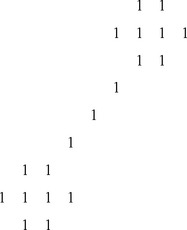
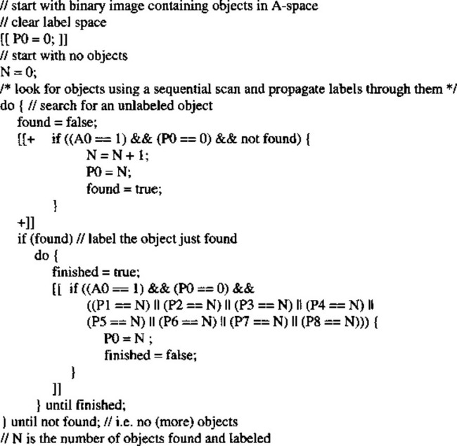
Now that we have a consistent definition of connectedness, we can unambiguously demarcate all objects in binary images and we should be able to devise algorithms for labeling them uniquely and counting them. Labeling may be achieved by scanning the image sequentially until a 1 is encountered on the first object. A note is then made of the scanning position, and a “propagation” routine is initiated to label the whole of the object with a 1. Since the original image space is already in use, a separate image space has to be allocated for labeling. Next, the scan is resumed, ignoring all points already labeled, until another object is found. This is labeled with a 2 in the separate image space. This procedure is continued until the whole image has been scanned and all the objects have been labeled (Fig. 6.1). Implicit in this procedure is the possibility of propagating through a connected object. Suppose at this stage that no method is available for limiting the field of the propagation routine, so that it has to scan the whole image space. Then the propagation routine takes the form:

Figure 6.1 A process in which all binary objects are labeled.

     (6.1)

the kernel of the do—until loop being expressed more explicitly as:

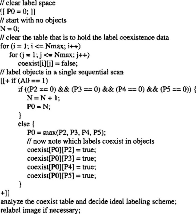
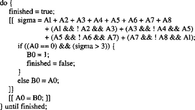
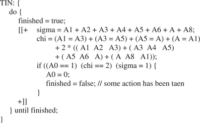
     (6.2)

At this stage a fairly simple type of algorithm for object labeling is obtained, as shown in Fig. 6.2; the [[+···+]] notation denotes a sequential scan over the image.

Figure 6.2 A simple algorithm for object labeling.

The above object counting and labeling routine requires a minimum of 2N +1 passes over the image space, and in practice the number will be closer to NW/2 where W is the average width of the objects. Hence, the algorithm is inherently inefficient. This prompts us to consider how the number of passes over the image can be reduced to save computation. One possibility would be to scan forward through the image, propagating new labels through objects as they are discovered. Although this would work mostly straightforwardly with convex objects, problems would be encountered with objects possessing concavities—for example, “U” shapes—since different parts of the same object would end with

different labels. Also, a means would have to be devised for coping with “collisions” of labels (e.g., the largest local label could be propagated through the remainder of the object: see Fig. 6.3). Then inconsistencies could be resolved by a reverse scan through the image. However, this procedure will not resolve all problems that can arise, as in the case of more complex (e.g., spiral) objects. In such cases, a general parallel propagation, repeatedly applied until no further labeling occurs, might be preferable—though as we have seen, such a process is inherently rather computationally intensive. However, it is implemented very conveniently on certain types of parallel SIMD (single instruction stream, multiple data stream) processors (see Chapter 28).

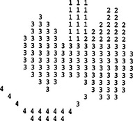
Figure 6.3 Labeling U-shaped objects: a problem that arises in labeling certain types of objects if a simple propagation algorithm is used. Some provision has to be made to accept “collisions” of labels, although the confusion can be removed by a subsequent stage of processing.

Ultimately, the least computationally intensive procedures for propagation involve a different approach: objects and parts of objects are labeled on a single sequential pass through the image, at the same time noting which labels coexist on objects. Then the labels are sorted separately, in a stage of abstract information processing, to determine how the initially rather ad hoc labels should be interpreted. Finally, the objects are relabeled appropriately in a second pass over the image. (This latter pass is sometimes unnecessary, since the image data are merely labeled in an overcomplex manner and what is needed is simply a key to interpret them.) The improved labeling algorithm now takes the form shown in Fig. 6.4. This algorithm with its single sequential scan is intrinsically far more efficient than the previous one, although the presence of particular dedicated hardware or a suitable SIMD processor might alter the situation and justify the use of alternative procedures.

Figure 6.4 The improved algorithm for object labeling.

Minor amendments to the above algorithms permit the areas and perimeters of objects to be determined. Thus, objects may be labeled by their areas or perimeters instead of by numbers representing their order of appearance in the image. More important, the availability of propagation routines means that objects can be considered in turn in their entirety—if necessary by transferring

them individually to separate image spaces or storage areas ready for unencumbered independent analysis. Evidently, if objects appear in individual binary spaces, maximum and minimum spatial coordinates are trivially measurable, centroids can readily be found, and more detailed calculations of moments (see below) and other parameters can easily be undertaken.

6.3.1 Solving the Labeling Problem in a More Complex Case

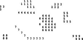
In this section we add substance to the all too facile statement at the end of Fig. 6.4: “analyze coexist table and decide ideal labeling scheme.” First, we have to make the task nontrivial by providing a suitable example. Figure 6.5 shows an example image, in which sequential labeling has been carried out in line with the algorithm of Fig. 6.4. However, one variation has been adopted—that of

Figure 6.5 Solving the labeling problem in a more complex case.

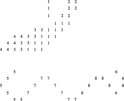
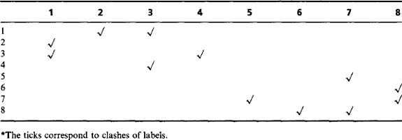
using a minimum rather than a maximum labeling convention, so that the values are in general slightly closer to the eventual ideal labels. (This also serves to demonstrate that there is not just one way of designing a suitable labeling algorithm.) The algorithm itself indicates that the coexist table should now appear as in Table 6.1. However, the whole process of calculating ideal labels can be made more efficient by inserting numbers instead of ticks, and also adding the right numbers along the leading diagonal, as in Table 6.2. For the same reason, the numbers below the leading diagonal, which are technically redundant, are retained here.

Table 6.1 Coexist table for the image of Fig. 6.4*

Table 6.2 Coexist table with additional numerical information*

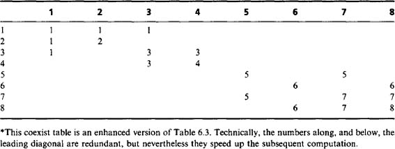
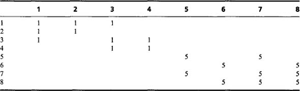
The next step is to minimize the entries along the individual rows of the table, as in Table 6.3; next we minimize along the individual columns (Table 6.4); and then we minimize along rows again (Table 6.5). This process is iterated to completion, which has already happened here after three stages of minimization. We can now read off the final result from the leading diagonal. Note that a further stage of computation is needed to make the resulting labels consecutive integers, starting with unity. However, the procedure needed to achieve this is much more basic and does not need to manipulate a 2-D table of data. This will be left as a simple programming task for the reader.

Table 6.3 Coexist table redrawn with minimized rows. At this stage the table is no longer symmetrical

Table 6.4 Coexist table redrawn again with minimized columns

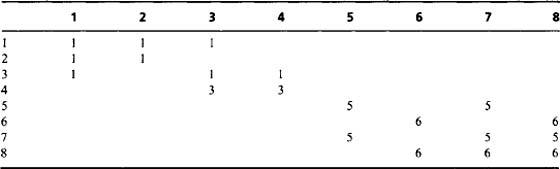
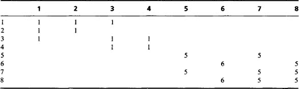
Table 6.5 Coexist table redrawn yet again with minimized rows. At this stage the table is in its final form and is once again symmetrical

At this point, some comment on the nature of the process described above will be appropriate. What has happened is that the original image data have effectively been condensed into the minimum space required to express the

labels—namely, just one entry per original clash. This explains why the table retains the 2-D format of the original image: lower dimensionality would not permit the image topology to be represented properly. It also explains why minimization has to be carried out, to completion, in two orthogonal directions. On the other hand, the particular implementation, including both above- and below-diagonal elements, is able to minimize computational overheads and finalize the operation in remarkably few iterations.

Finally, it might be felt that too much attention has been devoted to finding connected components of binary images. This is a highly important topic in practical applications such as industrial inspection, where it is crucial to locate all the objects unambiguously before they can individually be identified and scrutinized. In addition, Fig. 6.5 makes clear that it is not only U-shaped objects that give problems, but also those that have shape subtleties—as happens at the left of the upper object in this figure.

6.4 Metric Properties in Digital Images

Measurement of distance in a digital image is complicated by what is and what is not easy to calculate, given the types of neighborhood operations that are common in image processing. However, it must be noted that rigorous measures of distance depend on the notion of a metric. A metric is defined as a measure d(r_i, r_j) that fulfills three conditions:

Distance can be estimated accurately in a digital image using the Euclidean metric:

     (6.6)

However, it is interesting that the 8-connected and 4-connected definitions of connectedness given above also lead to measures that are metrics:

     (6.7)

and

     (6.8)

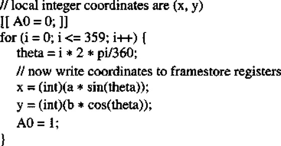
On the other hand, the latter two metrics are far from ideal in that they lead to constant distance loci that appear as squares and diamonds rather than as circles. In addition, it is difficult to devise other more accurate measures that fulfill the requirements of a metric. Clearly, this means that if we restrict ourselves to local neighborhood operations, we will not be able to obtain very high accuracy of measurement. Hence, if we require the maximum accuracy possible, it will be necessary to revert to using the Euclidean metric. For example, if we wish to draw an accurate ellipse, then we should employ some scheme such as that in Fig. 6.6 rather than attempting to employ neighborhood operations.

Figure 6.6 Routine for drawing an ellipse.

Similarly, if we find two features in an image and wish to measure their distance apart, it is trivial to do this by “abstract” processing using the two pairs of coordinates but difficult to do it efficiently by operations taking place entirely within image space. Nevertheless, it is useful to see how much can be achieved in image space. This aim has given rise to such approximations as the following widely used scheme for rapid estimation of the perimeter of an object: treat horizontal and vertical edges normally (i.e., as unit steps), but treat diagonal edges as times the step length. This rather limited approach (analyzed more fully in Chapter 7) is acceptable for certain simple recognition tasks.

6.5 Size Filtering

Although use of the d₄ and d₈ metrics is bound to lead to certain inaccuracies, it is useful to see what can be achieved with the use of local operations in binary images. This section studies how simple size filtering operations can be carried out, using merely local (3 × 3) operations. The basic idea is that small objects may be eliminated by applying a series of SHRINK operations. N SHRINK operations will eliminate an object (or those parts of an object) that are 2N or fewer pixels wide (i.e., across their narrower dimension). Of course this process shrinks all the objects in the image, but in principle a subsequent N EXPAND operation will restore the larger objects to their former size.

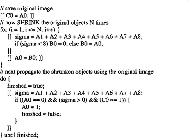
If complete elimination of small objects but perfect retention of larger objects is required, this will, however, not be achieved by the above procedure, since in many cases the larger objects will be distorted or fragmented by these operations (Fig. 6.7). To recover the larger objects in their original form, the proper approach is to use the shrunken versions as “seeds” from which to grow the originals via a propagation process. The algorithm of Fig. 6.8 is able to achieve this.

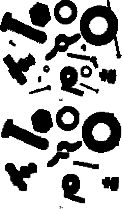
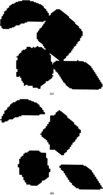
Figure 6.7 The effect of a simple size filtering procedure. When size filtering is attempted by a set of N SHRINK and N EXPAND operations, larger objects are restored aproximately to their original sizes, but their shapes frequently become distorted or even fragmented. In this example, (b) shows the effect of applying two SHRINK and then two EXPAND operations to the image in (a).

Figure 6.8 Algorithm for recovering original forms of shrunken objects.

Having seen how to remove whole (connected) objects that are everywhere narrower than a specified width, it is possible to devise algorithms for removing

any subset of objects that are characterized by a given range of widths. Large objects may be filtered out by first removing lesser-sized objects and then performing a logical masking operation with the original image, while intermediate-sized objects may be filtered out by removing a larger subset and then restoring small objects that have previously been stored in a separate image space. Ultimately, all these schemes depend on the availability of the propagation technique, which in turn depends on the internal connectedness of individual objects.

Finally, note that EXPAND operations followed by SHRINK (or thinning—see below) operations may be useful for joining nearby objects, filling in holes, and so on. Numerous refinements and additions to these simple techniques are possible. A particularly interesting one is to separate the silhouettes of touching objects such as chocolates by a shrinking operation. This then permits them to be counted reliably (Fig. 6.9).

Figure 6.9 Separation of touching objects by SHRINK operations. Here objects (chocolates) in (a) are shrunk (b) in order to separate them so that they may be counted reliably.

6.6 The Convex Hull and Its Computation

This section moves on to consider potentially more precise descriptions of shape, and in particular the convex hull. This is basically an analog descriptor of

shape, being defined (in two dimensions) as the shape enclosed by an elastic band placed around the object in question. The convex deficiency is defined as the shape that has to be added to a given shape to create the convex hull (Fig. 6.10).

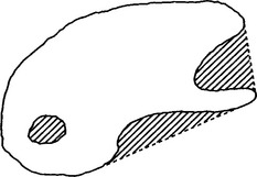
Figure 6.10 Convex hull and convex deficiency. The convex hull is the shape enclosed on placing an elastic band around an object. The shaded portion is the convex deficiency that is added to the shape to create the convex hull.

The convex hull may be used to simplify complex shapes to provide a rapid indication of the extent of an object. A particular application might be locating the hole in a washer or nut, since the hole is that part of the convex deficiency that is not adjacent to the background. In addition, the convexity or otherwise of a figure is determined by finding whether the convex deficiency is (to the required precision) an empty set. A fuller description of the shape of an object may be obtained by means of concavity trees. Here the convex hull of an object is first obtained with its convex deficiencies, next the convex hulls and deficiencies of the convex deficiencies are found, then the convex hulls and deficiencies of these convex deficiencies—and so on until all the derived shapes are convex. Thus, a tree is formed that can be used for systematic shape analysis and recognition (Fig. 6.11). We shall not dwell on this approach beyond noting its inherent utility and observing that at its core is the need for a reliable means of determining the convex hull of a shape.

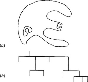
Figure 6.11 A simple shape and its concavity tree. The shape in (a) has been analyzed by repeated formation of convex hulls and convex deficiencies until all the constituent regions are convex (see text). The tree representing the entire process is shown in (b): at each node, the branch on the left is the convex hull, and the branches on the right are convex deficiencies.

A simple means of obtaining the convex hull (but not an accurate Euclidean one) is to repeatedly fill in the center pixel of all neighborhoods that exhibit a concavity, including each of the following:

until no further change occurs. If, as in the second example, a corner pixel in the neighborhood is 0 and is adjacent to two 1’s, it makes no difference to the 8-connectedness condition whether the corner is 0 or 1. Hence, we can pretend that it has been replaced by a 1. We then get a simple rule for determining whether to fill

in the center pixel. If there are four or more 1’s around the boundary of the neighborhood, then there is a concavity that must be filled in. This can be expressed as follows:

     (6.9)

However, the corner pixels may not in fact be present. It is therefore necessary to correct the routine as follows:²

     (6.10)

Finally, a complex convex hull algorithm (Fig. 6.12) requires the FILL routine to be included in a loop, with a suitable flag to test for completion. Note that the algorithm is forced to perform a final pass in which nothing happens. Although this seems to waste computation, it is necessary, for otherwise it will

Figure 6.12 The complete convex hull algorithm.

not be known that the process has run to completion. This situation arises repeatedly in this sort of work—there are seven examples in this chapter alone.

The shapes obtained by the above algorithm are actually overconvex and approximate to octagonal (or degenerate octagonal) shapes such as the following:

The method may be refined so that an approximately 16-sided polygon results (Hussain, 1988). This is achieved by forming the above “overconvex hull”; then forming an “underconvex hull” by finding the convex hull of the background with the constraint that it is permitted to eat into the convex deficiency but must not eat into the original object; then finding a median line (Fig. 6.13) between the over- and underconvex hulls by a suitable technique such as thinning (see Section 6.8).³

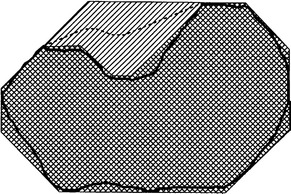
Figure 6.13 Finding an approximate convex hull using over- and underconvex hulls. The shaded region is the overconvex hull of the original shape, and the doubly shaded region is the underconvex hull. A (potentially) 16-sided approximation to the ideal convex hull is found by thinning the singly shaded region, as indicated by the dotted line.

Although such techniques making using of solely local operations are possible, and are ideally implemented on certain types of parallel processor (Hussain, 1988), they have only limited accuracy and can only be improved with considerable ingenuity. Ultimately, for connected objects, the alternative option of tracking around the perimeter of the object and deducing the position of the convex hull has to be adopted. The basic strategy for achieving this is simple—search for positions on the boundary that have common tangent lines. Note that changing from a body-oriented to a boundary-oriented approach can in principle save considerable computation. However, the details of this strategy are not trivial to implement because of the effects of spatial quantization which complicate these inherently simple analog ideas. Overall, there is no escape from the necessity to take connectedness fully into account. Hence, algorithms are required which can reliably track around object boundaries. This aspect of the problem is dealt with in a later section. Further details of convex hull algorithms based on this approach are not given here: the reader is referred to the literature for additional information (see, for example, Rutovitz, 1975).

Before leaving the topic of convex hull determination, a possible complication should be noted. This problem arises when the convex hulls of the individual objects overlap (though not the original objects). In this case, the final convex hull is undefined. Should it be the union of the separate convex hulls or the convex hull of their union? The local operator algorithm considered earlier will find the latter, whereas algorithms based on boundary tracking will find the former. In general, obtaining a convex hull from an original shape is not trivial, as tests must be incorporated to ensure that separate limbs are in all cases connected, and to ensure that the convex hulls of other objects are not inadvertently combined. Ultimately, such problems are probably best dealt with by transferring each object to its own storage area before starting convex hull computations (see also Section 6.3).

6.7 Distance Functions and Their Uses

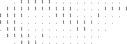
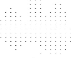
The distance function of an object is a very simple and useful concept in shape analysis. Essentially, each pixel in the object is numbered according to its distance from the background. As usual, background pixels are taken as 0’s; then edge pixels are counted as 1’s; object pixels next to 1’s become 2’s; next to those are the 3’s; and so on throughout all the object pixels (Fig. 6.14).

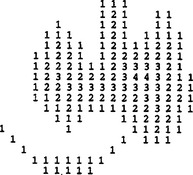
Figure 6.14 The distance function of a binary shape: the value at every pixel is the distance (in the d₈ metric) from the background.

The parallel algorithm of Fig. 6.15 finds the distance function of binary objects by propagation. Note that, as in the computation of convex hulls, this algorithm performs a final pass in which nothing happens. Again, this is inevitable if it is to be certain that the process runs to completion. An alternative way of propagating the distance function is shown in Fig. 6.16. Note the complication in ensuring completion of the procedure. If it could be assumed that N passes are needed for objects of known maximum width, then the algorithm would be simply:

Figure 6.15 A parallel algorithm for propagating distance functions.

Figure 6.16 An alternative parallel algorithm for propagating distance functions.

PPROP 3:

     (6.11)

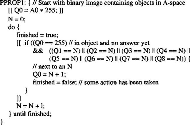
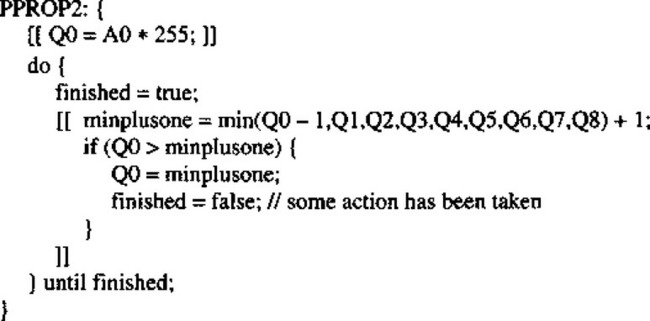
This routine operates entirely within a single image space and appears to be simpler and more elegant than PPROP1. Note, however, that in every pass

over the image it writes a value at every location, which under some circumstances could require more computation. (This is not true for PPROP1, which writes a value only at those object locations that are next to previously assigned values.) For SIMD parallel processing machines, which have a processing element at every pixel location, this is no problem, and PPROP3 may be more useful.

It is possible to perform the propagation of a distance function with far fewer operations if the process is expressed as two sequential operations, one being a normal forward raster scan and the other being a reverse raster scan:

     (6.12)

Note the compact notation being used to distinguish between forward and reverse raster scans over the image: [[+···+]] denotes a forward raster scan, while [[–···–]] denotes a reverse raster scan. A more succinct version of this algorithm is the following:

     (6.13)

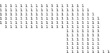
An interesting application of distance functions is that of data compression. To achieve it, operations are carried out to locate those pixels that are local maxima of the distance function (Fig. 6.17), since storing these pixel values and positions permits the original image to be regenerated by a process of downward propagation (see below). Note that although finding the local maxima of the distance function provides the basic information for data compression, the actual compression occurs only when the data are stored as a list of points rather than in the original picture format. In order to locate the local maxima, the following parallel routine may be employed:

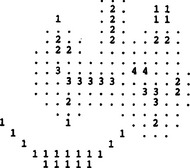
Figure 6.17 Local maxima of the distance function of the shape shown in Fig. 6.14, the remainder of the shape being indicated by dots and the background being blank. Notice that the local maxima group themselves into clusters, each containing points of equal distance function value, while clusters of different values are clearly separated.

     (6.14)

Alternatively, the compressed data can be transferred to a single image space:

     (6.15)

Note that the local maxima that are retained for the purpose of data compression are not absolute maxima but are maximal in the sense of not being adjacent to larger values. If this were not so, insufficient numbers of points would be retained for completely regenerating the original object. As a result, it is found that the absolute maxima group themselves into clusters of connected points, each cluster having a common distance value and being separated from points of different distance values (Fig. 6.17). Thus, the set of local maxima of an object is not a connected subset. This fact has an important bearing on skeleton formation (see below).

Having seen how data compression may be performed by finding local maxima ofthe distance function, it is relevant to consider a parallel downward propagation algorithm (Fig. 6.18) for recovering the shapes of objects from an image into which the values of the local maxima have been inserted. Note again that if it can be assumed that at most N passes are needed to propagate through objects of known maximum width, then the algorithm becomes simply:

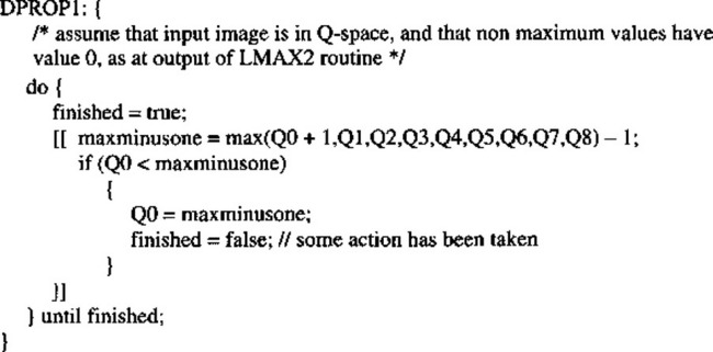
Figure 6.18 A parallel algorithm for recovering objects from the local maxima of the distance functions.

DPROP 2:

     (6.16)

Finally, although the local maxima of the distance function form a subset of points that may be used to reconstruct the object shape exactly, it is frequently possible to find a subset M of this subset that has this same property and thereby corresponds to a greater degree of data compression. This can be seen by appealing to Fig. 6.19. This is possible because although downward propagation from M permits the object shape to be recovered immediately, it does not also provide a correct set of distance function values. If required, these must be

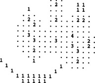
Figure 6.19 Minimal subset of points for object reconstruction. The numbered pixels may be used to reconstruct the entire shape shown in Fig. 6.14 and form a more economical subset than the set of local maxima of Fig. 6.17.

obtained by subsequent upward propagation. It turns out that the process of finding a minimal set of points M involves quite a complex and computationally intensive algorithm and is too specialized to describe in detail here (see Davies and Plummer, 1980).

6.8 Skeletons and Thinning

Like the convex hull, the skeleton is a powerful analog concept that may be employed for the analysis and description of shapes in binary images. A skeleton may be defined as a connected set of medial lines along the limbs of a figure. For example, in the case of thick hand-drawn characters, the skeleton may be the path actually traveled by the pen. The basic idea of the skeleton is that of eliminating redundant information while retaining only the topological information concerning the shape and structure of the object that can help with recognition. In the case of hand-drawn characters, the thickness of the limbs is taken to be irrelevant. It may be constant and therefore carry no useful information, or it may vary randomly and again be of no value for recognition (Fig. 1.2).

The skeleton definition presented earlier leads to the idea of finding the loci of the centers of maximal discs inserted within the object boundary. First, suppose the image space is a continuum. Then the discs are circles, and their centers form loci that may be modeled conveniently when object boundaries are approximated by linear segments. Sections of the loci fall into three categories:

Clearly, (1) and (2) are special forms of a more general case.

These ideas lead to unique skeletons for objects with linear boundaries, and the concepts are easily generalizable to curved shapes. This approach tends to give rather more detail than is commonly required, even the most obtuse corner having a skeleton line going into its apex (Fig. 6.20). Hence, a thresholding scheme is often employed, so that skeleton lines only reach into corners having a specified minimum degree of sharpness.

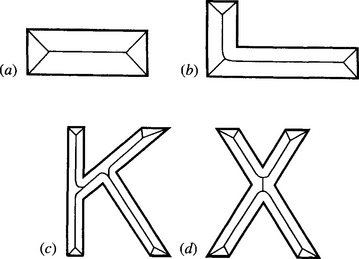
Figure 6.20 Four shapes whose boundaries consist entirely of straight-line segments. The idealized skeletons go right to the apex of each corner, however obtuse. In certain parts of shapes (b), (c), and (d), the skeleton segments are parts of parabolas rather than straight lines. As a result, the detailed shape of the skeleton (or the approximations produced by most algorithms operating in discrete images) is not exactly what might initially be expected or what would be preferred in certain applications.

We now have to see how the skeleton concept will work in a digital lattice. Here we are presented with an immediate choice: which metric should we employ? If we select the Euclidean metric, we are liable to engender a considerable computational load (although many workers do choose this option). If we select the d₈ metric we will immediately lose accuracy but the computational requirements should be more modest. (Here we do not consider the d₄ metric, since we are dealing with foreground objects.) In the following discussion we concentrate on the d₈ metric.

At this stage, some thought shows that the application of maximal discs in order to locate skeleton lines amounts essentially to finding the positions of local maxima of the distance function. Unfortunately, as seen in the previous section, the set of local maxima does not form a connected graph within a given object. Nor is it necessarily composed of thin lines, and indeed in places it may be 2 pixels wide. Thus, problems arise in trying to use this approach to obtain a

connected unit-width skeleton that can conveniently be used to represent the shape of the object. We shall return to this approach again below. Meanwhile, we pursue an alternative idea—that of thinning.

Thinning is perhaps the simplest approach to skeletonization. It may be defined as the process of systematically stripping away the outermost layers of a figure until only a connected unit-width skeleton remains (see, for example, Fig. 6.21). A number of algorithms are available to implement this process, with varying degrees of accuracy, and we will discuss how a specified level of precision can be achieved and tested for. First, however, it is necessary to discuss the mechanism by which points on the boundary of a figure may validly be removed in thinning algorithms.

Figure 6.21 Typical result of a thinning algorithm operating in a discrete lattice.

6.8.1 Crossing Number

The exact mechanism for examining points to determine whether they can be removed in a thinning algorithm must now be considered. This may be decided by reference to the crossing number χ (chi) for the 8 pixels around the outside of a particular 3 × 3 neighborhood. χ is defined as the total number of 0-to-1 and 1-to-0

transitions on going once round the outside of the neighborhood. This number is in fact twice the number of potential connections joining the remainder of the object to the neighborhood (Fig. 6.22). Unfortunately, the formula for χ is made more complex by the 8-connectedness criterion. Basically, we would expect:

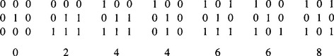
Figure 6.22 Some examples of the crossing number values associated with given pixel neighborhood configurations (0, background; 1, foreground).

     (6.17)

However, this is incorrect because of the 8-connectedness criterion. For example, in the case

the formula gives the value 4 for χ instead of 2. The reason is that the isolated 0 in the top right-hand corner does not prevent the adjacent 1’s from being joined. It is therefore tempting to use the modified formula:

     (6.18)

This too is wrong, however, since in the case

it gives the answer 2 instead of 4. It is therefore necessary to add four extra terms to deal with isolated 1’s in the corners:⁴

     (6.19)

This (now correct) formula for crossing number gives values 0, 2, 4, 6, or 8 in different cases (Fig. 6.22). The rule for removing points during thinning is that points may only be removed if they are at those positions on the boundary of an object where χ is 2: when χ is greater than 2, the point must be retained, for it forms a vital connecting point between two parts of the object. In addition, when χ is 0, it must be retained since removing it would create a hole.

Finally, one more condition must be fulfilled before a point can be removed during thinning—that the sum σ (sigma) of the eight pixel values around the outside of the 3 × 3 neighborhood (see Chapters 2) must not be equal to 1. The reason for this is to preserve line ends, as in the following cases:

If line ends are eroded as thinning proceeds, the final skeleton will not represent the shape of an object (including the relative dimensions of its limbs) at all accurately. (However, we might sometimes wish to shrink an object while preserving connectedness, in which case this extra condition need not be implemented.) Having covered these basics, we are now in a position to devise complete thinning algorithms.

6.8.2 Parallel and Sequential Implementations of Thinning

Thinning is “essentially sequential” in that it is easiest to ensure that connectedness is maintained by arranging that only one point may be removed at a time. As indicated earlier, this is achieved by checking before removing a point that has a crossing number of 2. Now imagine applying the “obvious” sequential algorithm of Fig. 6.23 to a binary image. Assuming a normal forward raster scan, the result of this process is to produce a highly distorted skeleton, consisting of lines along the right-hand and bottom edges of objects. It may now be seen that the χ = 2 condition is necessary but not sufficient, since it says nothing about the order in which points are removed. To produce a skeleton that is unbiased, giving a set of truly medial lines, it is necessary to remove points as evenly as possible around the object boundary. A scheme that helps with this involves a novel processing sequence: mark edge points on the first pass over an image; on the second pass, strip points sequentially as in the above algorithm, but only where they have already been marked; then mark a new set of edge points; then perform another stripping

Figure 6.23 An “obvious” sequential thinning algorithm.

pass; then finally repeat this marking and stripping sequence until no further change occurs. An early algorithm working on this principle is that of Beun (1973).

Although the novel sequential thinning algorithm described above can be used to produce a reasonable skeleton, it would be far better if the stripping action could be performed symmetrically around the object, thereby removing any possible skeletal bias. In this respect, a parallel algorithm should have a distinct advantage. However, parallel algorithms result in several points being removed at once. This means that lines 2 pixels wide will disappear (since masks operating in a 3 × 3 neighborhood cannot “see” enough of the object to judge whether or not a point may validly be removed), and as a result shapes can become disconnected. The general principle for avoiding this problem is to strip points lying on different parts of the boundary in different passes, so that there is no risk of causing breaks. This can be achieved in a large number of ways by applying different masks and conditions to characterize different parts of the boundary. If boundaries were always convex, the problem would no doubt be reduced; however, boundaries can be very convoluted and are subject to quantization noise, so the problem is a complex one. With so many potential solutions to the problem, we concentrate here on one that can conveniently be analyzed and that gives acceptable results.

The method discussed is that of removing north, south, east, and west points cyclically until thinning is complete. North points are defined as the following:

where × means either a 0 or a 1: south, east, and west points are defined similarly. It is easy to show that all north points for which χ = 2and σ ≠ 1 may be removed in parallel without any risk of causing a break in the skeleton—and similarly for south, east, and west points. Thus, a possible format for a parallel thinning algorithm in rectangular tessellation is the following:

     (6.20)

where the basic parallel routine for stripping “appropriate” north points is:

     (6.21)

(But extra code needs to be inserted to detect whether any changes have been made in a given pass over the image.)

Algorithms of the above type can be highly effective, although their design tends to be rather intuitive and ad hoc. In Davies and Plummer (1981), a great many such algorithms exhibited problems. Ignoring cases where the algorithm design was insufficiently rigorous to maintain connectedness, four other problems were evident:

1. The problem of skeletal bias.

2. The problem of eliminating skeletal lines along certain limbs.

3. The problem of introducing “noise spurs.”

4. The problem of slow speed of operation.

Problems (2) and (3) are opposites in many ways: if an algorithm is designed to suppress noise spurs, it is liable to eliminate skeletal lines in some circumstances. Contrariwise, if an algorithm is designed never to eliminate skeletal lines, it is unlikely to be able to suppress noise spurs. This situation arises because the masks and conditions for performing thinning are intuitive and ad hoc, and therefore have no basis for discriminating between valid and invalid skeletal lines. Ultimately this is because it is difficult to build overt global models of reality into purely local operators. In a similar way, algorithms that proceed with caution, that is, that do not remove object points in the fear of making an error or causing bias, tend to be slower in operation than they might otherwise be. Again, it is difficult to design algorithms that can make correct global decisions rapidly via intuitively designed local operators. Hence, a totally different approach is needed if solving one of the above problems is not to cause difficulties with the others. Such an alternative approach is discussed in the next section.

6.8.3 Guided Thinning

This section returns to the ideas discussed in the early part of Section 6.8, where it was found that the local maxima of the distance function do not form an ideal skeleton because they appear in clusters and are not connected. In addition, the clusters are often 2 pixels wide. On the plus side, the clusters are accurately in the correct positions and should therefore not be subject to skeletal bias. Hence, an ideal skeleton should result if (1) the clusters could be reconnected appropriately and (2) the resulting structure could be reduced to unit width. In this respect it should be noted that a unit width skeleton can only be perfectly unbiased where the object is an odd number of pixels wide: where the object is an even number of pixels wide, the unit-width skeleton is bound to be biased by 1/2 pixel, and the above strategy can give a skeleton that is as unbiased as is in principle possible.

A simple means of reconnecting the clusters is to use them to guide a conventional thinning algorithm (see Section 6.8.2). As a first stage, thinning is allowed to proceed normally but with the proviso that no cluster points may be removed. This gives a connected graph that is in certain places 2 pixels wide. Then a routine is applied to strip the graph down to unit width. At this stage, an unbiased skeleton (within 1/2 pixel) should result. The main problem here is the presence of noise spurs. The opportunity now exists to eliminate these systematically by applying suitable global rules. A simple rule is that of eliminating lines on the skeletal graph that terminate in a local maximum of value (say) 1 (or, better, stripping them back to the next local maximum), since such a local maximum corresponds to fairly trivial detail on the boundary of the object. Thus the level of detail that is ignored can be programmed into the system (Davies and Plummer, 1981). The whole guided thinning process is shown in Fig. 6.24.

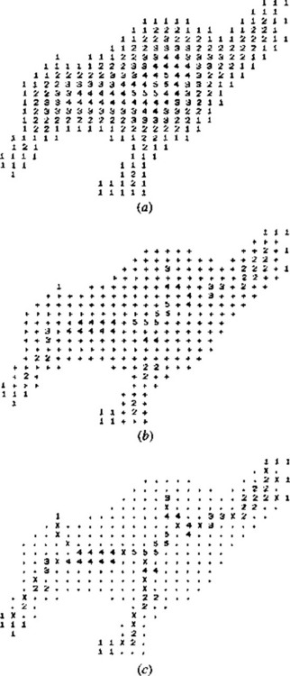
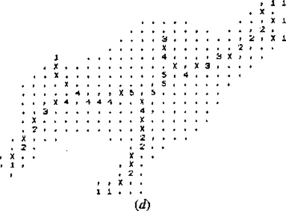
Figure 6.24 Results of a guided thinning algorithm: (a) distance function on the original shape; (b) set of local maxima; (c) set of local maxima now connected by a simple thinning algorithm; (d) final thinned skeleton. The effect of removing noise spurs systematically, by cutting limbs terminating in a 1 back to the next local maximum, is easily discernible from the result in (d): the general shape of the object is not perturbed by this process.

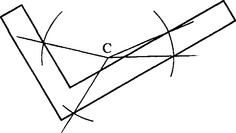
6.9 Some Simple Measures for Shape Recognition

Many simple tests of shape can be made to confirm the identity of products or to check for defects. These include measurements of product area and perimeter, length of maximum dimension, moments relative to the centroid, number and area of holes, area and dimensions of the convex hull and enclosing rectangle, number of sharp corners, number of intersections with a check circle and angles between intersections (Fig. 6.25), and numbers and types of skeleton nodes.

Figure 6.25 Rapid product inspection by polar checking.

The list would not be complete without mention of the widely used shape measure C = area/(perimeter)². This quantity is often called circularity or compactness, because it has a maximum value of 1/4π for a circle, decreases as shapes become more irregular, and approaches zero for long narrow objects. Alternatively, its reciprocal is sometimes used, being called complexity since it increases in size as shapes become more complex. Note that both measures are dimensionless, so that they are independent of size and are therefore sensitive only to the shape of an object. Other dimensionless measures of this type include rectangularity and aspect ratio.

All these measures have the property of characterizing a shape but not of describing it uniquely. Thus, it is easy to see that there are in general many different shapes having the same value of circularity. Hence, these rather ad hoc measures are on the whole less valuable than approaches such as skeletonization (Section 6.8) or moments (Section 6.10) that can be used to represent and reproduce a shape to any required degree of precision. Nevertheless, it should be noted that rigorous checking of even one measured number to high precision often permits a machined part to be identified positively.

6.10 Shape Description by Moments

Moment approximations provide one of the more obvious means of describing 2-D shapes and take the form of series expansions of the type:

     (6.22)

for a picture function f(x, y). Such a series may be curtailed when the approximation is sufficiently accurate. By referring axes to the centroid of the shape, moments can be constructed that are position-invariant. They can also be renormalized so that they are invariant under rotation and change of scale (Hu, 1962; see also Wong and Hall, 1978). The main value of using moment descriptors is that in certain applications the number of parameters may be made small without significant loss of precision—although the number required may not be clear without considerable experimentation. Moments can prove particularly valuable in describing shapes such as cams and other fairly round objects, although they have also been used in a variety of other applications including airplane silhouette recognition (Dudani et al., 1977).

6.11 Boundary Tracking Procedures

The preceding sections have described methods of analyzing shape on the basis of body representations of one sort or another—convex hulls, skeletons, moments, and so on. However, an important approach has so far been omitted—the use of boundary pattern analysis. This approach has the potential advantage of requiring considerably reduced computation, since the number of pixels to be examined is equal to the number of pixels on the boundary of any object rather than the much larger number of pixels within the boundary. Before proper use can be made of boundary pattern analysis techniques, the means must be found for tracking systematically around the boundaries of all the objects in an image. In addition, care must be taken not to ignore any holes that are present or any objects within holes.

In one sense, the problem has been analyzed already, in that the object labeling algorithm of Section 6.3 systematically visits and propagates through all objects in the image. All that is required now is some means of tracking around object boundaries once they have been encountered. Quite clearly, it will be useful to mark in a separate image space all points that have been tracked. Alternatively, an object boundary image may be constructed and the tracking performed in this space, all tracked points being eliminated as they are passed.

In the latter procedure, objects having unit width in certain places may become disconnected. Hence, we ignore this approach and adopt the previous one. There is still a problem when objects have unit-width sections, since these can cause badly designed tracking algorithms to choose a wrong path, going back around the previous section instead of on to the next (Fig. 6.26). To avoid this circumstance, it is best to adopt the following strategy:

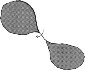
Figure 6.26 A problem with an oversimple boundary tracking algorithm. The boundary tracking procedure takes a shortcut across a unit-width boundary segment instead of continuing and keeping to the left path at all times.

Apart from necessary initialization at the start, a suitable tracking procedure is given in Fig. 6.27. Boundary tracking procedures such as this require careful coding. In addition, they have to operate rapidly despite the considerable amount of computation required for every boundary pixel. (See the amount of code within the main “do” loop of the procedure of Fig. 6.27.) For this reason it is normally best to implement the main direction-finding routine using lookup tables, or else using special hardware: details are, however, beyond the scope of this chapter.

Figure 6.27 Basic procedure for tracking around a single object.

Having seen how to track around the boundaries of objects in binary images, we are now in a position to embark on boundary pattern analysis. (See Chapter 7).

6.12 More Detail on the Sigma and Chi Functions

In this section, we present more explanation on the notation used in Sections 6.6 and 6.8.1. Essentially, this combines logical and unsigned integer arithmetic in a single expression relating to binary pixel values.

     (6.23)

In case of confusion, this statement may be written more conventionally in the form:

     (6.24)

Similarly, the statement:

     (6.25)

may be rewritten in the form:

     (6.26)

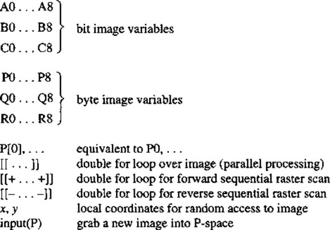
Note that, in general, declarations of variables are not given in the text but should be clear from the context. However, image variables are taken to be predeclared as bit or byte unsigned integers (see Fig. 6.28), bit variables being needed to hold shape information in binary images, and byte variables to hold information on up to 256 gray levels in gray-scale images (see Chapter 2).

Figure 6.28 Special syntax.

6.13 Concluding Remarks

This chapter has concentrated on rather traditional methods of performing image analysis—using image processing techniques. This has led naturally to area representations of objects, including, for example, moment and convex hull-based schemes, although the skeleton approach appeared as a rather special case in that it converts objects into graphical structures. An alternative schema is to represent shapes by their boundary patterns, after applying suitable tracking algorithms; this approach is considered in Chapter 7. Meanwhile, it should be noted that connectedness has been an underlying theme in the

present chapter, objects being separated from each other by regions of background, thereby permitting objects to be considered and characterized individually. Connectedness has been seen to involve rather more intricate computations than might have been expected, necessitating great care in the design of algorithms. This must partly explain why after so many years, new thinning algorithms are still being developed (e.g., Kwok, 1989; Choy et al., 1995). (Ultimately, these complexities arise because global properties of images are being computed by purely local means.)

Although boundary pattern analysis is in certain ways more attractive than region pattern analysis, this comparison cannot be divorced from considerations of the hardware the algorithms have to run on. In this respect, it should be noted that many of the algorithms of this chapter can be performed efficiently on SIMD processors, which have one processing element per pixel (see Chapter 28), whereas boundary pattern analysis will be seen to better match the capabilities of more conventional serial computers.

6.14 Bibliographical and Historical Notes

The development of shape analysis techniques has been extensive: hence, only a brief perusal of the history is attempted here. The all-important theory of connectedness and the related concept of adjacency in digital images were developed largely by Rosenfeld (see, e.g., Rosenfeld, 1970); for a review of this work, see Rosenfeld (1979). The connectedness concept led to the idea ofa distance function in a digital picture (Rosenfeld and Pfaltz, 1966, 1968) and the related skeleton concept (Pfaltz and Rosenfeld, 1967). However, the basic idea of a skeleton dates from the classic work by Blum (1967)—see also Blum and Nagel (1978). Important work on thinning has been carried out by Arcelli et al. (1975, 1981; Arcelli and di Baja, 1985) and parallels work by Davies and Plummer (1981). Note that the Davies-Plummer paper demonstrates a rigorous method for testing the results of any thinning algorithm, however generated, and in particular for detecting skeletal bias. More recently, Arcelli and Ramella (1995) have reconsidered the problem of skeletons in gray-scale images.

Returning momentarily to the distance function concept, which is of some importance for measurement applications, there have been important developments to generalize this concept and to make distance functions uniform and isotropic. See, for example, Huttenlocher et al. (1993).

Sklansky has carried out much work on convexity and convex hull determination (see, for example, Sklansky, 1970; Sklansky et al., 1976), while Batchelor (1979) developed concavity trees for shape description. Early work by Moore (1968) using shrinking and expanding techniques for shape analysis has been developed considerably by Serra and his co-workers (see, for example, Serra, 1986). Haralick et al. (1987) have generalized the underlying mathematical (morphological) concepts, including the case of gray-scale analysis. For more details, see Chapters 8. Use of invariant moments for pattern recognition dates from the two seminal papers by Hu (1961, 1962) and has continued unabated ever since. The field of shape analysis has been reviewed a number of times by Pavlidis (1977, 1978), and he has also drawn attention to the importance of unambiguous (“asymptotic”) shape representation schemes (Pavlidis, 1980).

Finally, the design of a modified crossing number χ_skel for the analysis of skeletal shape has not been considered until relatively recently. As pointed out in Section 6.8.5, χ_skel is different from χ because it judges the remaining (i.e., skeletal) points rather than points that might be eliminated from the skeleton (Davies and Celano, 1993b).

Most recently, skeletons have maintained their interest and utility, becoming if anything more precise by reference to exact analog shapes (Kégl and Krzyżak, 2002), and giving rise to the concept of a shock graph, which characterizes the result of the much earlier grass-fire transformation (Blum, 1967) more rigorously (Giblin and Kimia, 2003). Wavelet transforms have also been used to implement skeletons more accurately in the discrete domain (Tang and You, 2003). In contrast, shape matching has been carried out using self-similarity analysis coupled with tree representation—an approach that has been especially valuable for tracking articulated object shapes, including particularly human profiles and hand motions (Geiger et al., 2003). Finally, it is of interest to see graphical analysis of skeletonized hand-written character shapes performed taking account of catastrophe theory (Chakravarty and Kompella, 2003). This is relevant because (1) critical points—where points of inflection exist—can be deformed into pairs of points, each corresponding to a curvature maximum plus a minimum; (2) crossing of t’s can be actual or noncrossing; and (3) loops can turn into cusps or corners (many other possibilities also exist). The point is that methods are needed for mapping between variations of shapes rather than making snap judgments as to classification. (This corresponds to the difference between scientific understanding of process and ad hoc engineering.)

6.15 Problems

1. Write a routine for removing inconsistencies in labeling U-shaped objects by implementing a reverse scan through the image (see Section 6.3).

2. Write the full C++ routine required to sort the lists of labels, to be inserted at the end of the algorithm of Fig. 6.4.

3. Devise an algorithm for determining the “underconvex” hull described in Section 6.6.

4. Show that, as stated in Section 6.8.2 for a parallel thinning algorithm, all north points may be removed in parallel without any risk of causing a break in the skeleton.

5. Show that the convex-hull algorithm of Fig. 6.12 enlarges objects that may then coalesce. Find a simple means of locally inhibiting the algorithm to prevent objects from becoming connected in this way. Take care to consider whether a parallel or sequential process is to be used.

6. Describe methods for locating, labeling, and counting objects in binary images. You should consider whether methods based on propagation from a “seed” pixel, or those based on progressively shrinking a skeleton to a point, would provide the more efficient means for achieving the stated aims. Give examples for objects of various shapes.

7. (a) Give a simple one-pass algorithm for labeling the objects appearing in a binary image, making clear the role played by connectedness. Give examples showing how this basic algorithm goes wrong with real objects: illustrate your answer with clear pixel diagrams, that show the numbers of labels that can appear on objects of different shapes.

(b) Show how a table-oriented approach can be used to eliminate multiple labels in objects. Make clear how the table is set up and what numbers have to be inserted into it. Are the number of iterations needed to analyze the table similar to the number that would be needed in a multipass labeling algorithm taking place entirely within the original image? Consider how the real gain in using a table to analyze the labels arises.

8. (a) Using the normal notation for a 3 × 3 window:

work out the effect of the following algorithm on a binary image containing small foreground objects of various shapes:

until no further change;

(b) Show in detail how to implement the do… until no further change function in this algorithm.

9. (a) Give a simple algorithm operating in a 3 × 3 window for generating a rectangular convex hull around each object in a binary image. Include in your algorithm any necessary code for implementing the required do … until no further change function.

(b) A more sophisticated algorithm for finding accurate convex hulls is to be designed. Explain why this would employ a boundary tracking procedure. State the general strategy of an algorithm for tracking around the boundaries of objects in binary images and write a program for implementing it.

(c) Suggest a strategy for designing the complete convex hull algorithm and indicate how rapidly you would expect it to operate, in terms of the size of the image.

10. What are the problems in producing ideal object boundaries from the output of an edge detection operator? Show how disconnected edges might, in favorable conditions, be reconnected by a simple procedure such as extending lines in the same direction, until they meet other lines. Show that a better strategy is to join line ends only if the joining line would lie within a small angle of both line ends. What other factors should be taken into account in devising edge linking strategies? To what extent can any problems be overcome by any following algorithms, for example, Hough transforms?

11. (a) Explain the meaning of the term distance function. Give examples of the distance functions of simple shapes, including that shown in Fig. 6.P1.

Figure 6.P1

(b) Rapid image transmission is to be performed by sending only the coordinates and values of the local maxima of the distance functions. Give a complete algorithm for finding the local maxima of the distance functions in an image, and devise a further algorithm for reconstructing the original binary image.

(c) Discuss which of the following sets of data would give more compressed versions of the binary picture object shown in Fig. P1:

(i) the list of local maxima coordinates and values;

(ii) a list of the coordinates of the boundary points of the object;

(iii) a list consisting of one point on the boundary and the relative directions (each expressed as a 3-bit code) between each pair of boundary points on tracking round the boundary

12. (a) What is the distance function of a binary image? Illustrate your answer for the case where a 128 × 128 image P contains just the object shown in Fig. P2. How many passes of (i) a parallel algorithm and (ii) a sequential algorithm would be required to find the distance function of the image?

Figure 6.P2

(b) Give a complete parallel or sequential algorithm for finding the distance function, and explain how it operates.

(c)Image P is to be transmitted rapidly by determining the coordinates of locations where the distance function is locally maximum. Indicate the positions of the local maxima, and explain how the image could be reconstituted at the receiver.

(d)Determine the compression factor η if image P is transmitted in this way. Show that η can be increased by eliminating some of the local maxima before transmission, and estimate the resulting increase in η .

13. (a) The local maxima of the distance function can be defined in the following two ways:

(i) those pixels whose values are greater than those of all the neighboring pixels;

(ii) those pixels whose values are greater than or equal to the values of all the neighboring pixels. Which definition of the local maxima would be more useful for reproducing the original object shapes? Why is this?

(b) Give an algorithm that is capable of reproducing the original object shapes from the local maxima of the distance function, and explain how it operates.

(c) Explain the run-length encoding approach to image compression. Compare the run-length encoding and local maxima methods for compressing binary images. Explain why the one method would be expected to lead to a greater degree of compression with some types of images, while the other method would be expected to be better with other types of images.

14. (a) Explain how propagation of a distance function may be carried out using a parallel algorithm. Give in full a simpler algorithm that operates using two sequential passes over the image.

(b) It has been suggested that a four-pass sequential algorithm will be even faster than the two-pass algorithm, as each pass can use just a 1-D window involving at most three pixels. Write down the code for one typical pass of the algorithm.

(c) Estimate the approximate speeds of these three algorithms for computing the distance function, in the case of an N × N pixel image. Assume a conventional serial computer is used to perform the computation.

15. (a) A new wavefront method is devised for obtaining unbroken edges in grayscale images. It involves (i) detecting edges and thinning them to unit width, (ii) placing a 1 on the high-intensity side and a–1 on the other side of each edge point (in neither case affecting the edge points themselves, which are counted as having value 0), (iii) propagating distance function values from the 1’s and negative distance function values from the—1’s, and (iv) assigning 0 to any points that are adjacent to equal positive and negative values. Decide whether this specification is sufficient and whether any ambiguities remain. In the latter case, suggest suitable modifications to the procedure.

(b) Determine the effect of applying the complete algorithm. In your assessment of the algorithm, show what happens to edges that are initially (i) only slightly broken and (ii) widely spaced laterally. How could this algorithm be extended for use in practical situations?

16. Small dark insects are to be located among cereal grains. The insects approximate to rectangular bars of dimensions 20 by 7 pixels, and the cereal grains are approximately elliptical with dimensions 40 by 24 pixels. The proposed algorithm design strategy is: (i) apply an edge detector that will mark all the edge points in the image as 0’s in a 1’s background, (ii) propagate a distance function in the background region, (iii) locate the local maxima of the distance function, (iv) analyze the values of the local maxima, and (v) carry out necessary further processing to identify the nearly parallel sides of the insects. Explain how to design stages (iv) and (v) of the algorithm in order to identify the insects, ignoring the cereal grains. Assume that the image is not so large that the distance function will overflow the byte limit. Determine how robust the method will be if the edge is broken in a few places.

17. Give the general strategy of an algorithm for tracking around the boundaries of objects in binary images. If the tracker has reached a particular boundary point with crossing number χ = 2, such as

decide in which direction it should now proceed. Hence, give a complete procedure for determining the direction code of the next position on the boundary for cases where χ = 2. Take the direction codes starting from the current pixel (*) as being specified by the following diagram:

How should the procedure be modified for cases where χ = 2?

18. (a) Explain the principles involved in tracking around the boundaries of objects in binary images to produce reliable outlines. Outline an algorithm that can be used for this purpose, assuming it is to get its information from a normal 3 × 3 window.

(b) A binary image is obtained and the data in it are to be compressed as much as possible. The following range of modified images and datasets is to be tested for this purpose:

(i) the boundary image;

(ii) the skeleton image;

(iii) the image of the local maxima of the distance function;

(iv) the image of a suitably chosen subset of the local maxima of the distance function;

(v) a set of run-length data, that is, a series of numbers obtained by counting runs of 0’s, then runs of 1’s, then runs of 0’s, and so on, in a continuous line-by-line scan over the image.

In (i) and (ii) the lines may be encoded using chain code, that is, giving the coordinates of the first point met, and the direction of each subsequent point using the direction codes 1 to 8 defined relative to the current position C by:

With the aid of suitably chosen examples, discuss which of the methods of data compression should be most suitable for different types of data. Wherever possible, give numerical estimates to support your arguments.

(c) Indicate what you would expect to happen if noise were added to initially noise-free input images.