
CHAPTER 11 The Hough Transform and Its Nature
11.1 Introduction
As we have seen, the Hough transform (HT) is of great importance in detecting features such as lines and in circles, and in finding relevant image parameters (cf. the dynamic thresholding problem of Chapter 4). This makes it worthwhile to see the extent to which the method can be generalized so that it can detect arbitrary shapes. The work of Merlin and Farber (1975) and Ballard (1981) was crucial historically and led to the development of the generalized Hough transform (GHT). The GHT is studied in this chapter, first showing how it is implemented and then examining how it is optimized and adapted to particular types of image data. This requires us to go back to first principles, taking spatial matched filtering as a starting point.
Having developed the relevant theory, it is applied to the important case of line detection, showing in particular how detection sensitivity is optimized. Finally, the computational problems of the GHT are examined and fast HT techniques are considered.
11.2 The Generalized Hough Transform
This section shows how the standard Hough technique is generalized so that it can detect arbitrary shapes. In principle, it is trivial to achieve this objective. First, we need to select a localization point L within a template of the idealized shape. Then, we need to arrange it so that, instead of moving from an edge point a fixed distance R directly along the local edge normal to arrive at the center, as for circles, we move an appropriate variable distance R in a variable direction φ so as to arrive at L. R and φ are now functions of the local edge normal directions 6 (Fig. 11.1). Under these circumstances, votes will peak at the preselected object localization point L. The functions R(θ) and φ(θ) can be stored analytically in the computer algorithm, or for completely arbitrary shapes they may be stored as a lookup table. In either case, the scheme is beautifully simple in principle, but two complications arise in practice. The first develops because some shapes have features such as concavities and holes, so that several values of R and φ are required for certain values of 6 (Fig. 11.2). The second arises because we are going from an isotropic shape (a circle) to an anisotropic shape, which may be in a completely arbitrary orientation.
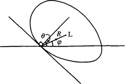
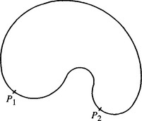
Figure 11.2 A shape exhibiting a concavity: certain values of 6 correspond to several points on the boundary and hence require several values of R and φ–as for points P1 and P2.
To cope with the first of these complications, the lookup table (usually called the R-table) must contain a list of the positions r, relative to L, of all points on the boundary of the object for each possible value of edge orientation 6 (or a similar effect must be achieved analytically). Then, on encountering an edge fragment in the image whose orientation is 6, estimates of the position of L may be obtained by moving a distance (or distances) R = - r from the given edge fragment. If the R-table has multivalued entries (i.e., several values of r for certain values of 6), only one of these entries (for given 6) can give a correct estimate of the position of L. However, at least the method is guaranteed to give optimum sensitivity, since all relevant edge fragments contribute to the peak at L in parameter space. This property of optimal sensitivity reflects the fact that the GHT is a form of spatial matched filter: this property is analyzed in more detail later in this chapter.
The second complication arises because any shape other than a circle is anisotropic. Since in most applications (including industrial applications such as automated assembly) object orientations are initially unknown, the algorithm has to obtain its own information on object orientation. This means adding an extra dimension in parameter space (Ballard, 1981). Then each edge point contributes a vote in each plane in parameter space at a position given by that expected for an object of given shape and given orientation. Finally, the whole of parameter space is searched for peaks, the highest points indicating both the locations of objects and their orientations. If object size is also a parameter, the problem becomes far worse; this complication is ignored here (although the method of Section 10.3 is clearly relevant).
The changes made in proceeding to the GHT leave it just as robust as the HT circle detector described previously. This gives an incentive to improve the GHT so as to limit the computational problems in practical situations. In particular, the size of the parameter space must be cut down drastically both to save storage and to curtail the associated search task. Considerable ingenuity has been devoted to devising alternative schemes and adaptations to achieve this objective. Important special cases are those of ellipse detection and polygon detection, and in each of these cases definite advances have been made. Ellipse detection is covered in Chapter 12 and polygon detection in Chapter 14. Here we proceed with some more basic studies of the GHT.
11.3 Setting Up the Generalized Hough Transform–Some Relevant Questions
The next few sections explore the theory underpinning the GHT, with the aim of clarifying how to optimize it systematically for specific circumstances. It is relevant to ask what is happening when a GHT is being computed. Although the HT has been shown to be equivalent to template matching (Stockman and Agrawala, 1977) and also to spatial matched filtering (Sklansky, 1978), further clarification is required. In particular, three problems (Davies, 1987c) need to be addressed, as follows:
1. The parameter space weighting problem. In introducing the GHT, Ballard mentioned the possibility of weighting points in parameter space according to the magnitudes of the intensity gradients at the various edge pixels. But when should gradient weighting be used in preference to uniform weighting?
2. The threshold selection problem. When using the GHT to locate an object, edge pixels are detected and used to compute candidate positions for the localization point L (see Section 11.2). To achieve this it is necessary to threshold the edge gradient magnitude. How should the threshold be chosen?
3. The sensitivity problem. Optimum sensitivity in detecting objects does not automatically provide optimum sensitivity in locating objects, and vice versa. How should the GHT be optimized for these two criteria?
To understand the situation and solve these problems, it is necessary to go back to first principles. A start is made on this in the next section.
11.4 Spatial Matched Filtering in Images
To discuss the questions posed in Section 11.3, it is necessary to analyze the process of spatial matched filtering. In principle, this is the ideal method of detecting objects, since it is well known (Rosie, 1966) that a filter that is matched to a given signal detects it with optimum signal-to-noise ratio under white noise1 conditions (North, 1943; Turin, 1960). (For a more recent discussion of this topic, see Davies, 1993a.)
Mathematically, using a matched filter is identical to correlation with a signal (or “template”) of the same shape as the one to be detected (Rosie, 1966). Here “shape” is a general term meaning the amplitude of the signal as a function of time or spatial location.
When applying correlation in image analysis, changes in background illumination cause large changes in signal from one image to another and from one part of an image to another. The varying background level prevents straightforward peak detection in convolution space. The matched filter optimizes signal-to-noise ratio only in the presence of white noise. Whereas this is likely to be a good approximation in the case of radar signals, this is not generally true in the case of images. For ideal detection, the signal should be passed through a “noise-whitening filter” (Turin, 1960), which in the case of objects in images is usually some form of high-pass filter. This filter must be applied prior to correlation analysis. However, this is likely to be a computationally expensive operation.
If we are to make correlation work with near optimal sensitivity but without introducing a lot of computation, other techniques must be employed. In the template matching context, the following possibilities suggest themselves:
1. Adjust templates so that they have a mean value of zero, to suppress the effects of varying levels of illumination in first order.
2. Break up templates into a number of smaller templates, each having a zero mean. Then as the sizes of subtemplates approach zero, the effects of varying levels of illumination will tend to zero in second order.
3. Apply a threshold to the signals arising from each of the subtemplates, so as to suppress those that are less than the expected variation in signal level.
If these possibilities fail, only two further strategies appear to be available:
4. Readjust the lighting system–an important option in industrial inspection applications, although it may provide little improvement when a number of objects can cast shadows or reflect light over each other.
5. Use a more “intelligent” (e.g., context-sensitive) object detection algorithm, although this will almost certainly be computationally intensive.
11.5 From Spatial Matched Filters to Generalized Hough Transforms
To proceed, we note that items (1) to (5) amount to a specification of the GHT. First, breaking up the templates into small subtemplates each having a zero mean and then thresholding them is analogous, and in many cases identical, to a process of edge detection (see, for example, the templates used in the Sobel and similar operators). Next, locating objects by peak detection in parameter space corresponds to the process of reconstructing whole template information from the subtemplate (edge location) data. The important point here is that these ideas reveal how the GHT is related to the spatial matched filter. Basically, the GHT can be described as a spatial matched filter that has been modified, with the effect of including integral noise whitening, by breaking down the main template into small zero-mean templates and thresholding the individual responses before object detection.
Small templates do not permit edge orientation to be estimated as accurately as large ones. Although the Sobel edge detector is in principle accurate to about 1° (see Chapter 5), there is a deleterious effect if the edge of the object is fuzzy. In such a case, it is not possible to make the subtemplates very small, and an intermediate size should be chosen which gives a suitable compromise between accuracy and sensitivity.
Employing zero-mean templates results in the absolute signal level being reduced to zero and only local relative signal levels being retained. Thus, the GHT is not a true spatial matched filter. In particular, it suppresses the signal from the bulk of the object, retaining only that near its boundary. As a result, the GHT is highly sensitive to object position but is not optimized for object detection.
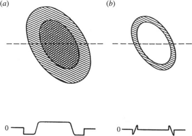
Thresholding of subtemplate responses has much the same effect as employing zero-mean templates, although it may remove a small proportion of the signal giving positional information. This makes the GHT even less like an ideal spatial matched filter and further reduces the sensitivity of object detection. The thresholding process is particularly important in the present context because it provides a means of saving computational effort without losing significant positional information. On its own, this characteristic of the GHT would correspond to a type of perimeter template around the outside of an object (see Fig. 11.3). This must not be taken as excluding all of the interior of the object, since any high-contrast edges within the object will facilitate location.
11.6 Gradient Weighting versus Uniform Weighting
The first problem described in Section 11.1 was that of how best to weight plots in parameter space in relation to the respective edge gradient magnitudes. To find an answer to this problem, it should now only be necessary to go back to the spatial matched filter case to find the ideal solution and then to determine the corresponding solution for the GHT in the light of the discussion in Section 11.4. First, note that the responses to the subtemplates (or to the perimeter template) are proportional to edge gradient magnitude. With a spatial matched filter, signals are detected optimally by templates of the same shape. Each contribution to the spatial matched filter response is then proportional to the local magnitude of the signal and to that of the template. In view of the correspondence between (1) using a spatial matched filter to locate objects by looking for peaks in convolution space and (2) using a GHT to locate objects by looking for peaks in parameter space, we should use weights proportional to the gradients of the edge points and proportional to the a priori edge gradients.
The choice of weighting is important for two reasons. First, the use of uniform weighting implies that all edge pixels whose gradient magnitudes are above threshold will effectively have them reduced to the threshold value, so that the signal will be curtailed. Accordingly, the signal-to-noise ratio of high-contrast objects could be reduced significantly. Second, the widths of edges of high-contrast objects will be broadened in a crude way by uniform weighting (see Fig. 11.4), but under gradient weighting this broadening will be controlled, giving a roughly Gaussian edge profile. Thus, the peak in parameter space will be narrower and more rounded, and the object reference point L can be located more easily and with greater accuracy. This effect is visible in Fig. 11.5, which also shows the relatively increased noise level that results from uniform weighting.
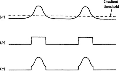
Figure 11.4 Effective gradient magnitude as a function of position within a section across an object of moderate contrast, thresholded at a fairly low level: (a) gradient magnitude for original image data and gradient thresholding level; (b) uniform weighting: the effective widths of edges are broadened rather crudely, adding significantly to the difficulty of locating the peak in parameter space; (c) gradient weighting: the position of the peak in parameter space can be estimated in a manner that is basically limited by the shape of the gradient profile for the original image data.
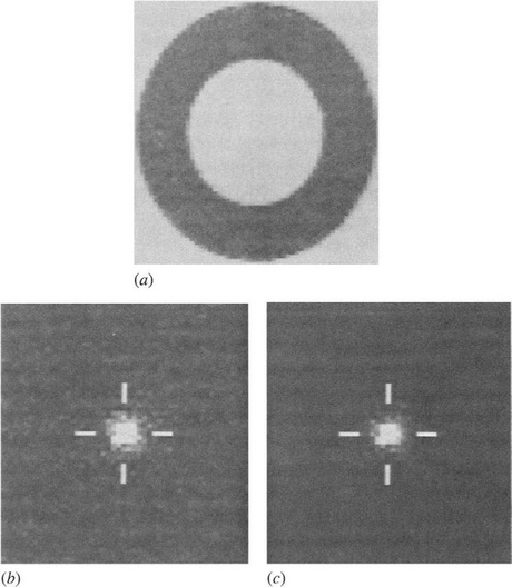
Figure 11.5 Results of applying the two types of weighting to a real image: (a) original image; (b) results in parameter space for uniform weighting; (c) results for gradient weighting. The peaks (which arise from the outer edges of the washer) are normalized to the same levels in the two cases. The increased level of noise in (b) is readily apparent. In this example, the gradient threshold is set at a low level (around 10% of the maximum level) so that low-contrast objects can also be detected.
Note also that low gradient magnitudes correspond to edges of poorly known location, while high values correspond to sharply defined edges. Thus, the accuracy of the information relevant to object location is proportional to the magnitude of the gradient at each of the edge pixels, and appropriate weighting should therefore be used.
11.6.1 Calculation of Sensitivity and Computational Load
In this subsection, we underline the above ideas by working out formulas for sensitivity and computational load. It is assumed that p objects of size around n × n are being sought in an image of size N × N.
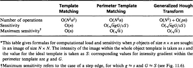
Correlation requires N2n2 operations to compute the convolutions for all possible positions of the object in the image. Using the perimeter template, we find that the number of basic operations is reduced to ~N2n, corresponding to the reduced number of pixels in the template. The GHT requires ~N2 operations to locate the edge pixels, plus a further pn operation to plot the points in parameter space.
The situation for sensitivity is rather different. With correlation, the results for n2 pixels are summed, giving a signal proportional to n2, although the noise (assumed to be independent at every pixel) is proportional to n. This is because of the well-known result that the noise powers of various independent noise components are additive (Rosie, 1966). Overall, this results in the signal-to-noise ratio being proportional to n. The perimeter template possesses only ~n pixels, and here the overall result is that the signal-to-noise ratio is proportional to ![]() . The situation for the GHT is inherently identical to that for the perimeter template method, as long as plots in parameter space are weighted proportional to edge gradient g multiplied by a priori edge gradient G. It is now necessary to compute the constant of proportionality a. Take s as the average signal, equal to the intensity (assumed to be roughly uniform) over the body of the object, and S as the magnitude of a full matched filter template. In the same units, g (and G)is the magnitude of the signal within the perimeter template (assuming the unit of length equals 1 pixel). Then α= 1/sS. This means that the perimeter template method and the GHT method lose sensitivity in two ways–first because they look at less of the available signal, and second because they look where the signal is low. For a high value of gradient magnitude, which occurs for a step edge (where most of the variation in intensity takes place within the range of 1 pixel), the values of g and G saturate out, so that they are nearly equal to s and S (see Fig. 11.6). Under these conditions the perimeter template method and the GHT have sensitivities that depend only on the value of n.
. The situation for the GHT is inherently identical to that for the perimeter template method, as long as plots in parameter space are weighted proportional to edge gradient g multiplied by a priori edge gradient G. It is now necessary to compute the constant of proportionality a. Take s as the average signal, equal to the intensity (assumed to be roughly uniform) over the body of the object, and S as the magnitude of a full matched filter template. In the same units, g (and G)is the magnitude of the signal within the perimeter template (assuming the unit of length equals 1 pixel). Then α= 1/sS. This means that the perimeter template method and the GHT method lose sensitivity in two ways–first because they look at less of the available signal, and second because they look where the signal is low. For a high value of gradient magnitude, which occurs for a step edge (where most of the variation in intensity takes place within the range of 1 pixel), the values of g and G saturate out, so that they are nearly equal to s and S (see Fig. 11.6). Under these conditions the perimeter template method and the GHT have sensitivities that depend only on the value of n.
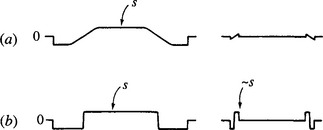
Figure 11.6 Effect of edge gradient on perimeter template signal: (a) low edge gradient: signal is proportional to gradient; (b) high edge gradient. Signal saturates at value of s.
Table 11.1 summarizes this situation. The oft-quoted statement that the computational load of the GHT is proportional to the number of perimeter pixels, rather than to the much greater number of pixels within the body of an object, is only an approximation. In addition, this saving is not obtained without cost. In particular, the sensitivity (signal-to-noise ratio) is reduced (at best) as the square root of object area/perimeter. (Note that area and perimeter are measured in the same units, so it is valid to find their ratio.)
Finally, the absolute sensitivity for the GHT varies as gG. As contrast changes so that g → g’, we see that gG → g’ G. That is, sensitivity changes by a factor ofg’/g. Hence, theory predicts that sensitivity is proportional to contrast. Although this result might have been anticipated, we now see that it is valid only under conditions of gradient weighting.
11.7 Summary
As described in this chapter, a number of factors are involved in optimizing the GHT, as follows.
1. (a) Each point in parameter space should be weighted in proportion to the intensity gradient at the edge pixel giving rise to it, and in proportion to the a priori gradient, if sensitivity is to be optimized, particularly for objects of moderate to high contrast.
2. The ultimate reason for using the GHT is to save computation. The main means by which this is achieved is by ignoring pixels having low magnitudes of intensity gradient. If the threshold of gradient magnitude is set too high, fewer objects are in general detected; if it is set too low, computational savings are diminished. Suitable means are required for setting the threshold, but little reduction in computation is possible if the highest sensitivity in a low-contrast image is to be retained.
3. The GHT is inherently optimized for the location of objects in an image but is not optimized for the detection of objects. It may therefore miss low-contrast objects which are detectable by other methods that take the whole area of an object into account. This consideration is often unimportant in applications where signal-to-noise ratio is less of a problem than finding objects quickly in an uncluttered environment.
Clearly, the GHT is a spatial matched filter only in a particular sense, and as a result it has suboptimal sensitivity. The main advantage of the technique is that it is highly efficient, with overall computational load in principle being proportional to the relatively few pixels on the perimeters of objects rather than to the much greater numbers of pixels within them. In addition, by concentrating on the boundaries of objects, the GHT retains its power to locate objects accurately. It is thus important to distinguish clearly between sensitivity in detecting objects and sensitivity in locating them.
11.8 Applying the Generalized Hough Transform to Line Detection
This section considers the effect of applying the GHT to line detection because it should be known how sensitivity may be optimized. Straight lines fall into the category of features such as concavities which give multivalued entries in the Rtable of the GHT–that is, certain values of 6 give rise to a whole set of values of r. Here we regard a line as a complete object and seek to detect it by a localization point at its midpoint M. Taking the line as having length S and direction given by unit vector u along its length, we find then that the transform of a general edge point E at e on the line is the set of points:2
or, more accurately (since the GHT is constructed so as to accumulate evidence for the existence of objects at particular locations), the transform function T(x) is unity at these points and zero elsewhere:3
Thus, each edge pixel gives rise to a line of votes in parameter space equal in length to the whole length of the line in the original shape. It is profitable to explore briefly why lines should have such an odd PSF, which contrasts strongly with the point PSF for circles. The reason is that a straight line is accurately locatable normal to its length, but inaccurately locatable along its length. (For an infinite line, there is zero accuracy of location along the length, and complete precision for location normal to the length.) Hence, lines cannot have a radially symmetrical PSF in a parameter space that is congruent to image space. (This solves a research issue raised by Brown, 1983.)
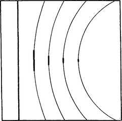
Circles and lines, however, do not form totally distinct situations but are two extremes of a more general situation. This is indicated in Fig. 11.7, which shows that progressively lowering the curvature for objects within the (limited) field of view leads to progressive lowering of the accuracy with which the object may be located in the direction along the visible part of the perimeter, but to no loss in accuracy in the normal direction.
11.9 The Effects of Occlusions for Objects with Straight Edges
As has been shown, the GHT gives optimum sensitivity of line detection only at the expense of transforming each edge point into a whole line of votes in parameter space. However, there is a resulting advantage, in that the GHT formulation includes a degree of intrinsic longitudinal localization of the line. We now consider this aspect of the situation more carefully.
While studying line transforms obtained using the GHT line parametrization scheme, it is relevant to consider what happens in situations where objects may be partly occluded. It will already be clear that sensitivity for line detection degrades gracefully, as for circle detection. But what happens to the line localization properties? The results are rather surprising and gratifying, as will be seen from Figs. 11.8-11.11 (Davies, 1989d). These figures show that the transforms of partly occluded lines have a distinct peak at the center of the line in all cases where both ends are visible and a flat-topped response otherwise, indicating the exact degree of uncertainty in the position of the line center (see Figs. 11.8 and 11.9). Naturally, this effect is spoiled if the line PSF that is used is of the wrong length, and then an uncertainty in the center position again arises (Fig. 11.10).
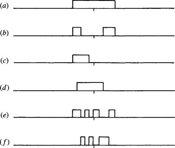
Figure 11.8 Various types of occlusions of a line: (a) original line; f) line with various types of occlusion (see text).
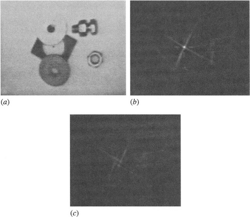
Figure 11.11 Location of a severely occluded rectangular object: (a) original image; (b) transform assuming that the short sides are oriented between 0 and π/2; (c) transform assuming that the short sides are oriented between π/2 and π. Note that the rectangular object is precisely located by the peak in (b), despite gross occlusions over much of its boundary. The fact that the peak in (b) is larger than those in (c) indicates the orientation of the rectangular object within π/2 (Davies, 1989c). (For further details, see Chapter 14.) Notice that occlusions could become so great that only one peak was present in either parameter plane and the remaining longer side was occluded down to the length of the shorter sides. There would then be insufficient information to indicate which range of orientations of the rectangle was correct, and an inherent ambiguity would remain.
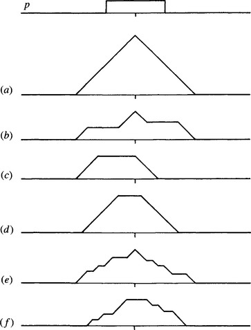
Figure 11.9 Transforms of a straight line and of the respective occluded variants shown in Fig. 11.8 (p, PSF). It is easy to see why response (a) takes the form shown. The result of correlating a signal with its matched filter is the autocorrelation function of the signal. Applying these results to a short straight line (Fig. 11.8 a) gives a matched filter with the same shape (p), and the resulting profile in convolution space is the autocorrelation function (a).
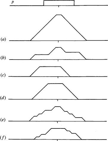
Figure 11.10 Transforms of a straight line and of the respective occluded variants shown in Fig. 11.8, obtained by applying a PSF that is slightly too long. The results should be compared with those in Fig. 11.9 (p, PSF).
Figure 11.11 shows a rectangular component being located accurately despite gross occlusions in each of its sides. The fact that L is independently the highest point in either branch of the transform at L is ultimately because two ends in each pair of parallel sides of the rectangle are visible.
Thus, the GHT parametrization of the line is valuable not only in giving optimum sensitivity in the detection of objects possessing straight edges, but it also gives maximum available localization of these straight edges in the presence of severe occlusions. In addition, if the ends of the lines are visible, then the centers of the lines are locatable precisely–a property that arises automatically as an integral part of the procedure, no specific line-end detectors being required. Thus, the GHT with the specified line parametrization scheme can be considered as a process that automatically takes possible occlusions into account in a remarkably “intelligent” way. Table 11.2 summarizes the differences between the normal and the GHT parametrizations of the straight line.
Table 11.2. Comparison between the two parametrizations of a straight line
| Normal parametrization | GHT parametrization |
| Localized relative to origin of coordinates | Localized relative to the line: independent of any origin |
| Basic localization point is foot-of-normal from origin | Basic localization point is midpoint of line |
| Provides no direct information on line’s longitudinal position | Provides definite information on line’s longitudinal position |
| Takes no account of length of line: this information not needed | Takes account of length of line: must be given this information, for optimal sensitivity |
| Not directly compatible with GHT | Directly compatible with GHT |
| Not guaranteed to give maximum sensitivity | Gives maximum sensitivity even when line is combined with other boundary segments |
11.10 Fast Implementations of the Hough Transform
As is now abundantly clear, the GHT has a severe weakness in that it demands considerable computation. The problem arises particularly with regard to the number of planes needed in parameter space to accommodate transforms for different object orientations and sizes. When line detection by the GHT is involved, an additional problem arises in that a whole line of votes is required for each edge pixel. Significant improvements in speed are needed before the GHT can achieve its potential in practical instances of arbitrary shapes. This section considers some important developments in this area.
The source of the computational problems of the HT is the huge size the parameter space can take. Typically, a single plane parameter space has much the same size as an image plane. (This will normally be so in those instances where parameter space is congruent to image space.) But when many planes are required to cope with various object orientations and sizes, the number of planes is likely to be multiplied by a factor of around 300 for each extra dimension. Hence, the total storage area will then involve some 10,000 million accumulator cells. Reducing the resolution might just make it possible to bring this down to 100 million cells, although accuracy will start to suffer. Further, when the HT is stored in such a large space, the search problem involved in locating significant peaks becomes formidable.
Fortunately, data are not stored at all uniformly in parameter space, which provides a key to solving both the storage and the subsequent search problem. The fact that parameter space is to be searched for the most prominent peaks–in general, the highest and the sharpest ones–means that the process of detection can start during accumulation. Furthermore, initial accumulation can be carried out at relatively low resolution, and then resolution can be increased locally as necessary in order to provide both the required accuracy and the separation of nearby peaks. In this context, it is natural to employ a binary splitting procedure–that is, to repeatedly double the resolution locally in each dimension of parameter space (e.g., the x dimension, the y dimension, the orientation dimension, and the size dimension, where these exist) until resolution is sufficient. A tree structure may conveniently be used to keep track of the situation.
Such a method (the “fast” HT) was developed by Li et al. (1985, 1986). Illingworth and Kittler (1987) did not find this method to be sufficiently flexible in dealing with real data and so produced a revised version (the “adaptive” HT) that permits each dimension in parameter space to change its resolution locally in tune with whatever the data demand, rather than insisting on some previously devised rigid structure. In addition, they employed a 9 × 9 accumulator array at each resolution rather than the theoretically most efficient 2 × 2 array, since this was found to permit better judgments to be made on the local data. This approach seemed to work well with fairly clean images, but later, doubts were cast on its effectiveness with complex images (Illingworth and Kittler, 1988). The most serious problem to be overcome here is that, at coarse resolutions, extended patterns of votes from several objects can overlap, giving rise to spurious peaks in parameter space. Since all of these peaks have to be checked at all relevant resolutions, the whole process can consume more computation than it saves. Optimization in multiresolution peak-finding schemes is complex4 and data-dependent, and so discussion is curtailed here. The reader is referred to the original research papers (Li et al., 1985, 1986; Illingworth and Kittler, 1987) for implementation details.
An alternative scheme is the hierarchical HT (Princen et al., 1989a); so far it has been applied only to line detection. The scheme can most easily be envisaged by considering the foot-of-normal method of line detection described in Section 9.3. Rather small subimages of just 16 × 16 pixels are taken first of all, and the foot-of-normal positions are determined. Then each foot-of-normal is tagged with its orientation, and an identical HT procedure is instigated to generate the foot-of-normal positions for line segments in 32 × 32 subimage. This procedure is then repeated as many times as necessary until the whole image is spanned at once. The paper by Princen et al. discusses the basic procedure in detail and also elaborates necessary schemes for systematically grouping separate line segments into full-length lines in a hierarchical context. (In this way the work extends the techniques described in Section 9.4.) Successful operation of the method requires subimages with 50% overlap to be employed at each level. The overall scheme appears to be as accurate and reliable as the basic HT method but does seem to be faster and to require significantly less storage.
11.11 The Approach of Gerig and Klein
The Gerig and Klein approach was first demonstrated in the context of circle detection but was only mentioned in passing in Chapter 10. This is because it is an important approach that has much wider application than merely to circle detection. The motivation for it has already been noted in the previous section–namely, the problem of extended patterns of votes from several objects giving rise to spurious peaks in parameter space.
Ultimately, the reason for the extended pattern of votes is that each edge point in the original image can give rise to a very large number of votes in parameter space. The tidy case of detection of circles of known radius is somewhat unusual, as will be seen particularly in the chapters on ellipse detection and 3-D image interpretation. Hence, in general most of the votes in parameter space are in the end unwanted and serve only to confuse. Ideally, we would like a scheme in which each edge point gives rise only to the single vote corresponding to the localization point of the particular boundary on which it is situated. Although this ideal is not initially realizable, it can be engineered by the “back-projection” technique of Gerig and Klein (1986). Here all peaks and other positions in parameter space to which a given edge point contributes are examined, and a new parameter space is built in which only the vote at the strongest of these peaks is retained. (There is the greatest probability, but no certainty, that it belongs to the largest such peak.) This second parameter space thus contains no extraneous clutter, and so weak peaks are found much more easily, giving objects with highly fragmented or occluded boundaries a much greater chance of being detected. Overall, the method avoids many of the problems associated with setting arbitrary thresholds on peak height–in principle no thresholds are required in this approach.
The scheme can be applied to any HT detector that throws multiple votes for each edge point. Thus, it appears to be widely applicable and is capable of improving robustness and reliability at an intrinsic expense of approximately doubling computational effort. (However, set against this is the relative ease with which peaks can be located–a factor that is highly data-dependent.) Note that the method is another example in which a two-stage process is used for effective recognition.
Other interesting features of the Gerig and Klein method must be omitted here for reasons of space, although it should be pointed out that, rather oddly, the published scheme ignores edge orientation information as a means of reducing computation.
11.12 Concluding Remarks
The Hough transform was introduced in Chapter 9 as a line detection scheme and then used in Chapter 10 for detecting circles. In those chapters it appeared as a rather cunning method for aiding object detection. Although it was seen to offer various advantages, particularly in its robustness in the face of noise and occlusion, its rather novel voting scheme appeared to have no real significance. The present chapter has shown that, far from being a trick method, the HT is much more general an approach than originally supposed. Indeed, it embodies the properties of the spatial matched filter and is therefore capable of close-to-optimal sensitivity for object detection. Yet this does not prevent its implementation from entailing considerable computational load, and significant effort and ingenuity have been devoted to overcoming this problem, both in general and in specific cases. The general case is tackled by the schemes discussed in the previous two sections, while two specific cases–those of ellipse and polygon detection–are considered in detail in the following chapters. It is important not to underestimate the value of specific solutions, both because such shapes as lines, circles, ellipses, and polygons cover a large proportion of (or approximations to) manufactured objects, and because methods for coping with specific cases have a habit (as for the original HT) of becoming more general as workers see possibilities for developing the underlying techniques. For further discussion and critique of the whole HT approach, see Chapter 29.
The development of the Hough transform may appear somewhat arbitrary. However, this chapter has shown that it has solid roots in matched filtering. In turn, this implies that votes should be gradient weighted for optimal sensitivity. Back-projection is another means of enhancing the technique to make optimal use of its capability for spatial search.
11.13 Bibliographical and Historical Notes
Although the HT was introduced as early as 1962, a number of developments–including especially those of Merlin and Farber (1975) and Kimme et al. (1975)–were required before the GHT was developed in its current standard form (Ballard, 1981). By that time, the HT was already known to be formally equivalent to template matching (Stockman and Agrawala, 1977) and to spatial matched filtering (Sklansky, 1978). However, the questions posed in Section 11.3 were only answered much later (Davies, 1987c), the necessary analysis being reproduced in Sections 11.4-11.7. Sections 11.8-11.11 reflect Davies’ work (1987d,j, 1989d) on line detection by the GHT, which was aimed particularly at optimizing sensitivity of line detection, although deeper issues of tradeoffs between sensitivity, speed, and accuracy are also involved.
By 1985, the computational load of the HT became the critical factor preventing its more general use–particularly as the method could by that time be used for most types of arbitrary shape detection, with well-attested sensitivity and considerable robustness. Preliminary work in this area had been carried out by Brown (1984), with the emphasis on hardware implementations of the HT. Li, et al. (1985, 1986) showed the possibility of much faster peak location by using parameter spaces that are not uniformly quantized. This work was developed further by Illingworth and Kittler (1987) and others (see, for example, Illingworth and Kittler, 1988; Princen et al., 1989a,b; Davies, 1992h). The future will undoubtedly bring many further developments. Unfortunately, however, the solutions may be rather complex and difficult (or at least tedious) to program because of the contextual richness of real images. However, an important development has been the randomized Hough transform (RHT), pioneered by Xu and Oja (1993) among others: it involves casting votes until specific peaks in parameter space become evident, thereby saving unnecessary computation.
Accurate peak location remains an important aspect of the HT approach. Properly, this is the domain of robust statistics, which handles the elimination of outliers (of which huge numbers arise from the clutter of background points in digital images–see Appendix A). However, Davies (1992g) has shown a computationally efficient means of accurately locating HT peaks. He has also found why in many cases peaks may appear narrower than a priori considerations would indicate (Davies, 1992b). Kiryati and Bruckstein (1991) have tackled the aliasing effects that can arise with the Hough transform and that have the effect of cutting down accuracy.
Over time, the GHT approach has been broadened by geometric hashing, structural indexing, and other approaches (e.g., Lamdan and Wolfson, 1988; Gavrila and Groen, 1992; Califano and Mohan, 1994). At the same time, a probabilistic approach to the subject has been developed (Stephens, 1991) which puts it on a firmer footing (though rigorous implementation would in most cases demand excessive computational load). Finally, Grimson and Huttenlocher (1990) warn against the blithe use of the GHT for complex object recognition tasks because of the false peaks that can appear in such cases, though their paper is probably overpessimistic. For further review of the state of the subject up to 1993, see Leavers (1992, 1993).
In various chapters of Part 2, the statement has been made that the Hough transform5 carries out a search leading to hypotheses that should be checked before a final decision about the presence of an object can be made. However, Princen et al. (1994) show that the performance of the HT can be improved if it is itself regarded as a hypothesis testing framework. This is in line with the concept that the HT is a model-based approach to object location. Other studies have recently been made about the nature of the HT. In particular, Aguado et al. (2000) consider the intimate relationship between the Hough transform and the principle of duality in shape description. The existence of this relationship underlines the importance of the HT and provides a means for a more general definition of it. Kadyrov and Petrou (2001) have developed the trace transform, which can be regarded as a generalized form of the Radon transform, which is itself closely related to the Hough transform.
Other workers have used the HT for affine-invariant search. Montiel et al. (2001) made an improvement to reduce the incidence of wrong evidence in the gathered data, while Kimura and Watanabe (2002) made an extension for 2-D shape detection that is less sensitive to the problems of occlusion and broken boundaries. Kadyrov and Petrou (2002) have adapted the trace transform to cope with affine parameter estimation.
In a generalization of the work of Atherton and Kerbyson (1999), and of Davies (1987c) on gradient weighting (see Section 11.6), Anil Bharath and his colleagues have examined how to optimize the sensitivity of the HT (private communication, 2004). Their method is particularly valuable in solving the problems of early threshold setting that limit many HT techniques. Similar sentiments have emerged in a different way in the work of Kesidis and Papamarkos (2000), which maintains the gray-scale information throughout the transform process, thereby leading to more exact representations of the original images.
Olson (1999) has shown that localization accuracy can be improved efficiently by transferring local error information into the HT and handling it rigorously. An important finding is that the HT can be subdivided into many subproblems without a decrease of performance. This finding is elaborated in a 3-D model-based vision application where it is shown to lead to reduced false positive rates (Olson, 1998). Wu et al. (2002) extend the 3-D possibilities further by using a 3-D HT to find glasses. First, a set of features are located that lie on the same plane, and this is then interpreted as the glasses rim plane. This approach allows the glasses to be separated from the face, and then they can be located in their entirety.
van Dijck and van der Heijden (2003) develop the geometric hashing method of Lamdan and Wolfson (1988) to perform 3-D correspondence matching using full 3-D hashing. This method is found to have advantages in that knowledge of 3-D structure can be used to reduce the number of votes and spurious matches. Tytelaars et al. (2003) describe how invariant-based matching and Hough transforms can be used to identify regular repetitions in planes appearing within visual (3-D) scenes in spite of perspective skew. The overall system has the ability to reason about consistency and is able to cope with periodicities, mirror symmetries, and reflections about a point.
Finally, in an unusual 3-D application, Kim and Han (1998) use the Hough transform to analyze scenes taken from a line-scan camera in linear motion. The images are merged to form a “slit image,” which is partitioned into segmented regions, each directly related to a simple surface. In this representation, the correspondence problem (Chapter 16) is reduced to the simpler process ofdetecting straight lines using the HT.
1 White noise is noise that has equal power at all frequencies. In image science, white noise is understood to mean equal power at all spatial frequencies. The significance of this is that noise at different pixels is completely uncorrelated but is subject to the same gray-scale probability distribution–that is, it has potentially the same range of amplitudes at all pixels.
2 Here it is convenient to employ standard mathematical set notation, the curly brackets being used to represent a set of points.
3 The symbol ∈ means “is a member of the following set”; the symbol ∉ means “is not a member of the following set.” (In this case, the point x is or is not within the given range.)
4 Ultimately, the problem of system optimization for analysis of complex images is a difficult one, since in conditions of low signal-to-noise ratio even the eye may find it difficult to interpret an image and may “lock on” to an interpretation that is incorrect. It is worth noting that in general image interpretation work there are many variables to be optimized–sensitivity, efficiency/speed, storage, accuracy, robustness, and so on–and it is seldom valid to consider any of these individually. Often tradeoffs between just two such variables can be examined and optimized, but in real situations multivariable tradeoffs should be considered. This is a very complex task, and it is one of the purposes of this book to show clearly the serious nature of these types of optimization problems, although at the same time it can only guide the reader through a limited number of basic optimization processes.
5 A similar statement can be made in the case of graph matching methods such as the maximal clique approach to object location (see Chapter 15).