3.1 Introduction

In this chapter the discussion is extended to noise suppression and enhancement in gray-scale images. Although these types of operations can for the most part be avoided in industrial applications of vision, it is useful to examine them in some depth because of their wide use in a variety of other image processing applications and because they set the scene for much of what follows. In addition, some fundamental issues come to light which are of vital importance.

It has already been seen that noise can arise in real images; hence it is necessary to have sound techniques for suppressing it. Commonly, in electrical engineering applications, noise is removed by means of low-pass or other filters that operate in the frequency domain (Rosie, 1966). Applying these filters to 1-D time-varying analog signals is straightforward, since it is necessary only to place them at suitable stages in the sequence of black boxes through which the signals pass. For digital signals, the situation is more complicated, since first the frequency transform of the signal must be computed, then the low-pass filter applied, and finally the signal obtained from the modified transform by converting back to the time domain. Thus, two Fourier transforms have to be computed, although modifying the signal while it is in the frequency domain is a straightforward task (Fig. 3.1). It is by now well known that the amount of processing involved in computing a discrete Fourier transform of a signal represented by N samples is of order N² (we shall write this as O(N²)), and that the amount of computation can be cut down to O(N log₂N) by employing the fast Fourier transform (FFT) (Gonzalez and Woods, 1992). This then becomes a practical approach for the elimination of noise.

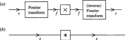
Figure 3.1 Low-pass filtering for noise suppression: s, spatial domain; f, spatial frequency domain; x, multiplication by low-pass characteristic; *, convolution with Fourier transform of low-pass characteristics. (a) Low-pass filtering achieved most simply, by a process of multiplication in the (spatial) frequency domain; (b) low-pass filtering achieved by a process of convolution. Note that (a) may require more computation overall because of the two Fourier transforms that have to be performed.

When applying these ideas to images, we must first note that the signal is a spatial rather than a time-varying quantity and must be filtered in the spatial frequency domain. Mathematically, this makes no real difference, but there are nevertheless significant problems. First, there is no satisfactory analog shortcut, and the whole process has to be carried out digitally. (Here we ignore optical processing methods despite their obvious power, speed, and high resolution, because they are by no means trivial to marry with digital computer technology; also, while there is much ongoing research in this area, it is difficult to anticipate the future position with any accuracy.) Second, for an N × N pixel image, the number of operations required to compute a Fourier transform is O(N³) and the FFT only reduces this to O(N² log₂ N), so the amount of computation is quite considerable. (Here it is assumed that the 2-D transforms are implemented by successive passes of 1-D transforms: see Gonzalez and Woods, 1992.) Note also that two Fourier transforms are required for the purpose of noise suppression (Fig. 3.1). Nevertheless, in many imaging applications it is worth proceeding in this way, not only so that noise can be removed but also so that TV scan lines and other artifacts can be filtered out. This situation particularly applies in remote sensing and space technology. However, in industrial applications the emphasis is always on real-time processing; in many cases, therefore, it is not practicable to remove noise by spatial frequency domain operations. A secondary problem is that low-pass filtering is suited to removing Gaussian noise but distorts the image if it is used to remove impulse noise.

Section 3.2 discusses Gaussian smoothing in both the spatial frequency and the spatial domains. The subsequent three sections introduce median filters, mode filters, and then general rank order filters, and contrast their main properties and uses. In Section 3.6 consideration is given to reducing computational load—with particular reference to the median filter. Section 3.7 introduces the sharp-unsharp masking technique, which provides a rather simple route to image enhancement. Then follow a number of sections that concentrate on the edge shifts produced by the various filters. In the case of the median filter, the discrete theory (Section 3.9) is much more exact than the continuum model (Section 3.8). All edge shifts are quite small, except for rank order filters (Section 3.12); these are treated fairly fully because of their relevance to widely used morphological operators (Chapter 8) where the shifts are turned to advantage.

3.2 Noise Suppression by Gaussian Smoothing

Low-pass filtering is normally thought of as the elimination of signal components with high spatial frequencies; it is therefore natural to carry it out in the spatial frequency domain. Nevertheless, it is possible to implement it directly in the spatial domain. That this is possible is due to the well-known fact (Rosie, 1966) that multiplying a signal by a function in the spatial frequency domain is equivalent to convolving it with the Fourier transform of the function in the spatial domain (Fig. 3.1). If the final convolving function in the spatial domain is sufficiently narrow, then the amount of computation involved will not be excessive. In this way, a satisfactory implementation of the low-pass filter can be sought. It now remains to find a suitable convolving function.

If the low-pass filter is to have a sharp cutoff, then its transform in image space will be oscillatory. An extreme example is the sinc (sin x/x) function, which is the spatial transform of a low-pass filter of rectangular profile (Rosie, 1966). It turns out that oscillatory convolving functions are unsatisfactory since they can introduce halos around objects, hence distorting the image quite grossly. Marr and Hildreth (1980) suggested that the right types of filters to apply to images are those that are well behaved (nonoscillatory) both in the frequency and in the spatial domain. Gaussian filters are able to fulfill this criterion optimally: they have identical forms in the spatial and spatial frequency domains. In 1-D these forms are

     (3.1)

     (3.2)

Thus, the type of spatial convolving operator required for the purpose of noise suppression by low-pass filtering is one that approximates to a Gaussian profile. Many such approximations appear in the literature; these vary with the size of the neighborhood chosen and in the precise values of the convolution mask coefficients.

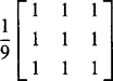
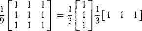
One of the most common masks is the following one, first introduced in Chapter 2, which is used more for simplicity of computation than for its fidelity to a Gaussian profile:

Another commonly used mask, which approximates more closely to a Gaussian profile, is the following:

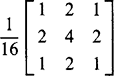
In both cases, the coefficients that precede the mask are used to weight all the mask coefficients. As mentioned in Section 2.2.3, these weights are chosen so that applying the convolution to an image does not affect the average image intensity. These two convolution masks probably account for over 80% of all discrete approximations to a Gaussian. Notice that as they operate within a 3 × 3 neighborhood, they are reasonably narrow and hence incur a relatively small computational load.

Let us next study the properties of this type of operator, deferring for now consideration of Gaussian operators in larger neighborhoods. First, imagine such an operator applied to a noisy image whose intensity is inherently uniform. Then clearly noise is suppressed, as it is now averaged over 9 pixels. This averaging model is obvious for the first of the two masks above but in fact applies equally to the second mask, once it is accepted that the averaging effect is differently distributed in accordance with the improved approximation to a Gaussian profile.

Although this example shows that noise is suppressed, it will be plain that the signal is also affected. This problem arises only where the signal is initially nonuniform. Indeed, if the image intensity is constant, or if the intensity map approximates to a plane, there is again no problem. However, if the signal is uniform over one part of a neighborhood and rises in another part of it, as is bound to occur adjacent to the edge of an object, then the object will make itself felt at the center of the neighborhood in the filtered image (see Fig. 3.2). As a result, the edges of objects become somewhat blurred. Looking at the operator as a “mixing operator” that forms a new picture by mixing together the intensities of pixels fairly close to each other, it is intuitively obvious why blurring occurs.

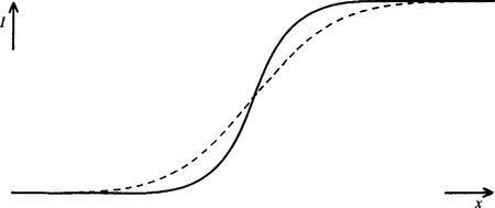
Figure 3.2 Blurring of object edges by simple Gaussian convolutions. The simple Gaussian convolution can be regarded as a gray-scale neighborhood “mixing” operator, hence explaining why blurring arises.

It is also apparent, from a spatial frequency viewpoint, why blurring should occur. Basically, we are aiming to give the signal a sharp cutoff in the spatial frequency domain, and as a result it will become slightly blurred in the spatial domain. Clearly, the blurring effect can be reduced by using the narrowest possible approximation to a Gaussian convolution filter, but at the same time the noise suppression properties of the filter are lessened. Assuming that the image was initially digitized at roughly the correct spatial resolution, it will not normally be appropriate to smooth it using convolution masks larger than 3 × 3 or at most 5 × 5 pixels. (Here we ignore methods of analyzing images that use a number of versions of the image with different spatial resolutions: see, for example, Babaud et al., 1986.)

Overall, low-pass filtering and Gaussian smoothing are not appropriate for the applications considered here because they introduce blurring effects. Notice also that where interference occurs, which can give rise to impulse or “spike” noise (corresponding to a number of individual pixels having totally the wrong intensities), merely averaging this noise over a larger neighborhood can make the situation worse, since the spikes will be smeared over a sizable number of pixels and will distort the intensity values of all of them. This consideration is important, leading naturally to the concepts of limit and median filtering.

3.3 Median Filters

The idea explored here is to locate those pixels in the image which have extreme and therefore highly improbable intensities and to ignore their actual intensities, replacing them with more suitable values. This is akin to drawing a graph through a set of plots and ignoring those plots that are evidently a long way from the best fit curve. An obvious way of using this technique is to apply a “limit” filter that prevents any pixel from having an intensity outside the intensity range of its neighbors:

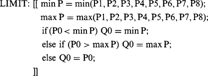     (3.3)

To develop this technique, it is necessary to examine the local intensity distribution within a particular neighborhood. Points at the extremes of the distribution are quite likely to have arisen from impulse noise. Not only is it sensible to eliminate these points, as in the limit filter, but it is reasonable to try taking the process further, removing equal areas at either end of the distribution and ending with the median. Thus, we arrive at the median filter, which takes all the local intensity distributions and generates a new image corresponding to the set of median values. As the preceding argument indicates, the median filter is excellent at impulse noise suppression; this is amply confirmed in practice (see Fig. 3.3).

Figure 3.3 Effect of applying a 3 × 3 median filter to the image of Fig. 2.1a. Note the slight loss of fine detail and the rather “softened” appearance of the whole image.

In view of the blurring caused by Gaussian smoothing operators, it is pertinent to ask whether the median filter also induces blurring. Figure 3.3 shows that any blurring is only marginal, although some slight loss of fine detail takes place, which can give the resulting pictures a “softened” appearance. Theoretical discussion of this point is deferred for now. The lack of blur makes good the main deficiency of the Gaussian smoothing filter and results in the median filter being almost certainly the single most widely used filter in general image processing applications.

The median filter may be implemented in many ways: Figure 3.4 reproduces only an obvious algorithm that essentially implements the above description. The notation of Chapter 2 is used but is augmented suitably to permit the nine pixels in a 3 × 3 neighborhood to be accessed in turn with a running suffix (specifically, P0 to P8 are written as P[m], where m runs from 0 to 8).

Figure 3.4 An implementation of the median filter.

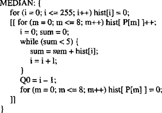
The operation of the algorithm is as follows: first, the histogram array is cleared and the image is scanned, generating a new image in Q-space; next, for each neighborhood, the histogram of intensity values is constructed; then the median is found; and, finally, points in the histogram array that have been incremented are cleared. This last feature eliminates the need to clear the whole histogram and hence saves computation. Further savings could be made by finding the extreme intensity values and limiting the search for the median to this range. Unlike the general situation when the median of a distribution is being located, only one (half-) scan through the distribution is required, since the total area is known in advance (in this case it is 9).

As is clear from the above, methods of computing the median involve pixel intensity sorting operations. If a bubble sort (Gonnet, 1984) were used for this purpose, then up to O(n⁴) operations would be required for an n × n neighborhood, compared with some 256 operations for the histogram method we have described. Thus, sorting methods such as the bubble sort are faster for small neighborhoods where n is 3 or 4 but not for neighborhoods where n is greater than about 5, or where pixel intensity values are more restricted.

Much of the discussion of the median filter in the literature is concerned with saving computation (Narendra, 1978; Huang et al., 1979; Danielsson, 1981). In particular, it has been observed that, on proceeding from one neighborhood to the next, relatively few new pixels are encountered. Thus, the new median value can be found by updating the old value rather than starting from scratch (Huang et al., 1979).

3.4 Mode Filters

Having considered the mean and the median of the local intensity distribution as candidate intensity values for noise smoothing filters, we also find it relevant to consider the mode of the distribution. Indeed, we might imagine that this is, if anything, more important than the mean or the median, since the mode represents the most probable value of any distribution.

A tedious problem arises, however, as soon as we attempt to apply this idea. The local intensity distribution is calculated from relatively few pixel intensity values (Fig. 3.5). This means that instead of a smooth intensity distribution whose mode is easily located, we are almost certain to have a multimodal distribution whose highest point does not indicate the position of the underlying mode. Clearly, the distribution needs to be smoothed out considerably before the mode is computed. Another tedious problem is that the width of the distribution varies widely from neighborhood to neighborhood (e.g., from close to zero to close to 256), so that it is difficult to know quite how much to smooth the distribution in any instance. For these reasons, it is likely to be better to choose an indirect measure of the position of the mode rather than to attempt to measure it directly.

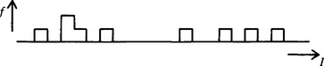
Figure 3.5 The sparse nature of the local intensity histogram for a small neighborhood. This situation clearly causes significant problems for estimation of the mode. It also has definite implications for rigorous estimation of the underlying median, assuming that the observed intensities are only noisy samples of the ideal intensity pattern (see Section 3.8.4).

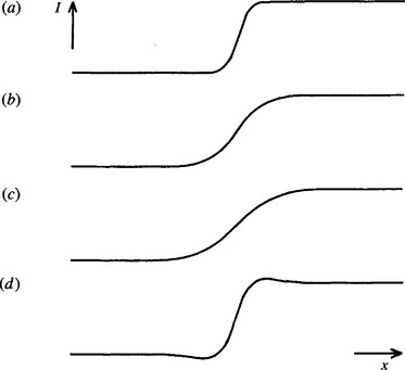
The position of the mode can be estimated with reasonable accuracy once the median has been located (Davies, 1984a, 1988c). To understand the technique, it is necessary to consider how local intensity distributions of various sorts arise in practical situations. At most positions in an image, variations in pixel intensity are generated by steady changes in background illumination, or by steady variations in surface orientation, or else by noise. Thus, a symmetrical unimodal local intensity distribution is to be expected. It is well known that the mean, median, and mode are coincident in such cases. More problematic is what happens to the intensity variation near the edge of an object in the image. Here the local intensity distribution is unlikely to be symmetrical, and, more important, it may not even be unimodal. In fact, near an edge the distribution is in general inherently bimodal, since the neighborhood contains pixels with intensities corresponding to the values they would have on either side of the edge (Fig. 3.6). Considering the image as a whole, this will be the most likely alternative to a symmetrical unimodal distribution; any further possibilities such as trimodal distributions are rare and of varied causes (e.g., odd glints on the edges of metal objects) and are outside the scope of the present discussion.¹

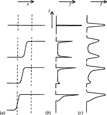
Figure 3.6 Local models of image data near the edge of an object: (a) cross sections of an edge falling in the vicinity of a filter neighborhood; (b) corresponding local intensity distributions when very little image noise is present; (c) situation when the noise level is increased.

If the neighborhood straddles an edge and the local intensity distribution is bimodal, the larger peak position should clearly be selected as the most probable intensity value. A good strategy for finding the larger peak is to eliminate the smaller peak. If we knew the position of the mode, we could find where to truncate the smaller peak by first finding which extreme of the distribution was closer to the mode, and then moving an equal distance to the opposite side of the mode (Fig. 3.7). Since we start off not knowing the position of the mode, one option is to use the position of the median as an estimator of the position of the mode, and then to use that position to find where to truncate the distribution. Since the three means invariably take the order mean, median, and mode (see Fig. 3.8), except when distributions are badly behaved or multimodal, it turns out that this method is cautious in the sense that it truncates less of the distribution than the required amount: this makes it a safe method to use. When we now find the median of the truncated distribution, the position is much closer to the mode than the original median was, a good proportion of the second peak having been removed (Fig. 3.9). Iteration could be used to find an even closer approximation to the position of the mode. However, the results show that the method gives a marked enhancement in the image even when this is not done (Fig. 3.10).

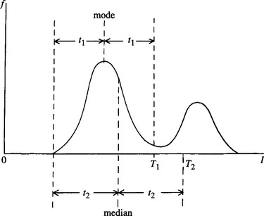
Figure 3.7 Rationale for the method of truncation. The obvious position at which to truncate the distribution is T₁. Since the position of the mode is not initially known, it is suboptimal but safe to truncate instead at T₂.

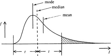
Figure 3.8 Relative positions of the mode, median, and mean for a typical unimodal distribution. This ordering is unchanged for a bimodal distribution, as long as it can be approximated by two Gaussian distributions of similar width.

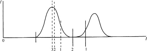
Figure 3.9 Iterative truncation of the local intensity distribution. Here the median converges on the mode within three iterations of the truncation procedure. This is possible since at each stage the mode of the new truncated distribution remains the same as that of the previous distribution.

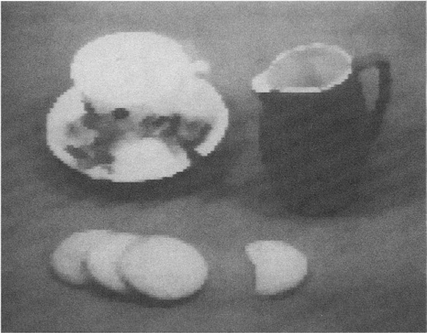
Figure 3.10 Effect of a single application of 3 × 3 truncated median filter to the image of Fig. 2.1a

What has been achieved by the above procedure? When we compare the results of applying a median filter and the new filter (which we call a truncated median filter, for it is not a true mode filter—see below), we find that whereas the median filter is highly successful at removing noise, the new filter not only removes noise but also enhances the image so that edges are made sharper. By reference to Fig. 3.11 it is quite easy to see why this should happen. Basically, at a location even very slightly to one side of an edge, a majority of the pixel intensities contribute to the larger peak and the filter ignores the pixel intensities contributing to the smaller peak. Thus, the filter makes an informed binary choice about which side of the edge it is on. At first this seems to mean that it pushes a nearby edge further away. However, it must be remembered that it actually “pushes the edge away” from both sides, and the result is that its sides are made sharper and object outlines are crispened up. Particularly striking is the effect of applying this filter to an image a number of times, when objects start to become segmented into regions of fairly uniform intensity (Fig. 3.12). The complete algorithm for achieving this is outlined in Fig. 3.13.

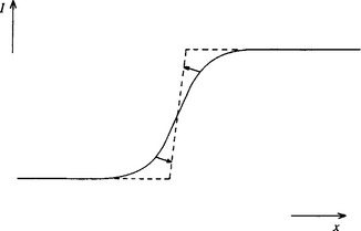
Figure 3.11 Image enhancement performed by the mode filter. Here the onset of the edge is pushed laterally by the action of the mode filter within one neighborhood. Since the same happens from the other side within an adjacent neighborhood, the actual position of the edge is unchanged in first order. The overall effect is to sharpen the edge.

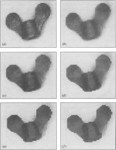
Figure 3.12 Results of repeated action of the truncated median filter: (a) the original, moderately noisy picture; (b) effect of a 3 × 3 median filter; (c)-(f) effect of 1-4 passes of the basic truncated median filter, respectively.

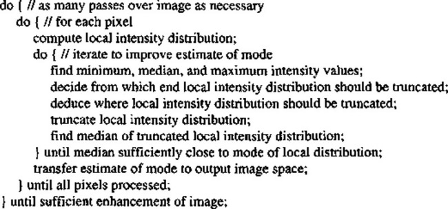
Figure 3.13 Outline of algorithm for implementing the truncated median filter. In this algorithm (i) The outermost and innnermost loops can normally be omitted (i.e., they need to be executed once only). (ii) The final estimate of the position of the mode can be performed by simple averaging instead of computing the median: this has been found to save computation with negligible loss of accuracy. (iii) Instead of the minimum and maximum intensity values, the positions of the outermost octiles (for example) may be used to give more stable estimates of the extremes of the local intensity distribution.

We have dealt with this problem at some length for several reasons. First, it seems that the mode filter has not hitherto received the attention it deserves. Second, the median filter seems to be used fairly universally, often without very much justification or thought. Third, all these filters show what markedly different characteristics are available merely by analyzing the contents of the local intensity distribution and ignoring totally where in the neighborhood the different intensities appear. It is perhaps remarkable that there is sufficient information in the local intensity distribution for this to be possible. All this shows the danger of applying operators that have been derived in an ad hoc manner without first making a specification of what is required and then designing an operator with the required characteristics. In fact, it appears that if we want a filter that has maximum impulse noise suppression capability, then we should use a median filter; and if we want a filter that enhances images by sharpening edges, then we should use a mode or truncated median filter. (Note that the truncated median filter should in some ways be an improvement on the mode filter in that it is more cautious when very close to an edge transition, where noise prevents an exact judgement from being made as to which side of the edge a pixel is on: see Davies, 1984a, 1988c.)

While considering enhancement, attention has been restricted to filters based on the local intensity distribution; many filters enhance images without the aid of the local intensity distribution (Lev et al., 1977; Nagao and Matsuyama, 1979), but they are not within the scope of this chapter. Note that the method of “sharp-unsharp masking” (Section 3.7) performs an enhancement function, although its main purpose is to restore images that have inadvertently become blurred, for example, by a hazy atmosphere or defocussed camera.

Finally, although this section has concentrated on the gray-scale properties of mode filters, Charles and Davies (2003a, 2004) have recently shown how to devise versions of the mode filter that operate on color images. Typical results are shown in Fig. 2.8. In addition, Fig. 2.9 shows that the mode filter has the hitherto unexpected property of being able to eliminate very large amounts of impulse noise from images—significantly more than a median filter—in spite of being designated as an image enhancement filter.

3.5 Rank Order Filters

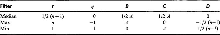
The principle employed in rank order filters is to take all the intensity values in a given neighborhood; place these in order of increasing value; and finally select the rth of the n values and return this value as the filter local output value. Clearly, n rank order filters can be specified in terms of the value r that is used, but these filters are all intrinsically nonlinear; that is, the output intensity cannot be expressed as a linear sum of the component intensities within the neighborhood. In particular, the median filter (for which r = (n + 1)/2, and which is only defined if n is odd²) does not normally give the same output image as a mean filter. Indeed, it is well known that the mean and median of a distribution are in general only coincident for symmetrical distributions. Note that minimum and maximum filters (corresponding to r = 1 and r = n, respectively) are also often classed as morphological filters (see Chapter 8).

3.6 Reducing Computational Load

Significant efforts have been made to speed the operation of the Gaussian filter since implementations in large neighborhoods require considerable amounts of computation (Wiejak et al., 1985). For example, smoothing images using a 30 × 30 Gaussian convolution mask in an image of 256 × 256 pixels involves 64 million basic operations. For such a basic operation as smoothing, this is unacceptable. However, the amount of computation can be cut down drastically, since a 2-D Gaussian convolution can be factorized into two 1-D Gaussian convolutions which can be applied in turn:

     (3.4)

The decomposition is rigorously provable and is not an approximation; we shall refer to this below in the context of the median filter. Meanwhile, the decompositions for the two 3 × 3 Gaussian filters we met earlier are:

     (3.5)

and

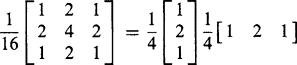     (3.6)

Overall, this approach replaces a single n × n operator whose load is O(n²) with two operators of load O(n), and for n > 3 there are always worthwhile savings. Ignoring scanning and other overheads we are summarize the situation in Table 3.1, the final column of which represents the saving factor.

Table 3.1. Savings achieved by factorizing an n × n Gaussian operator

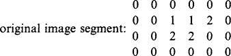
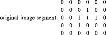
It turns out that it is not possible to decompose the median filter in the same way without making approximations. However, it is quite common to try to perform a similar function by applying two 1-D median filters in turn (Narendra, 1978). Although the effect is similar in its outlier rejection properties to the corresponding 2-D median filter, by appealing to specific examples of image data it is simple to show that the two are not formally equivalent. An instance in which the same effect is obtained by a 3 × 3 median filter or by 3 × 1 and 1 × 3 median filters applied in either order is the following:

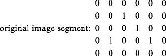
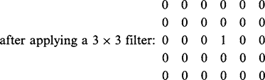
In this case, all the 1’s immediately disappear after applying a 3 × 3ora3×1ora 1 × 3 median filter. In the following instance, the situation is slightly more complex:

after applying a 3 × 1 and then a 1 × 3 filter:

after applying a 3 × 1 and then a 1 × 3 filter:

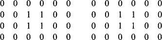
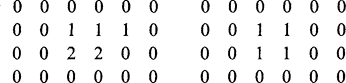
The following case tests the situation more thoroughly and is one of the simplest for which the three final image segments are all different:

after applying a 3 × 1 and then a 1 × 3 filter:

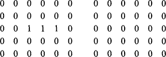
after applying a 1 × 3 and then a 3 × 1 filter:

In general, spots and streaks not more than one pixel wide are eliminated quite effectively by the original or by the separated forms of the filter. Larger filters should effectively eliminate wider spots and streaks, although exact functional equivalence between the original and its separated forms is not to be expected, as has been indicated.

Finally, the problem of inexact decomposition is not an exclusive property of nonlinear filters: many linear filters cannot be decomposed exactly either, because the number of independent coefficients in an n × n mask is n ² which is much greater than the number in an n × 1 or 1 × n component mask.

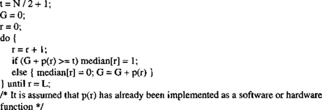
3.6.1 A Bit-based Method for Fast Median Filtering

A number of other means have been employed to speed the operation of the median filter. Of especial interest is the bit-based method of Ataman et al. (1980), since it is surprisingly simple, yet highly effective. Space does not permit a full account of the method to be given here, so a simplified version retaining the same main underlying principle is given.

The basic idea derives from the observation that only the most significant bit (MSB) of each of the original numbers is relevant for computing the MSB of the median. This suggests that it ought to be possible to determine the median in a number of operations of the order of the number of bits required to represent the original numbers. Since pixel intensities are frequently represented by just 6 to 8 bits of data, this makes the idea a particularly attractive one for further development in image processing applications.

To proceed, the discussion is specialized to the case where the numbers involved are the N pixel intensities within a given neighborhood, each represented by L bits, and t is the number of the median in the ordered sequence of the pixel intensities (so that t = N /2 +1). Bits are here labeled from the MSB to the LSB in the order 1,2,…, L in which they will be examined. Finally, p(r) denotes the number of pixels for which the rth bit is 1, while the first r—1 bits are identical to those of the median (as so far determined during the processing).

In this notation, the MSB of the median will be 1 if p(1) is at least t and 0 otherwise:

     (3.7)

It is relevant to what follows to note that if p(1)< t, this identifies p(1) pixel intensities as being greater than the median: otherwise none is so identified.

This simple result is somewhat tricky to generalize; in fact, it is now necessary to restate the problem. At any stage, let us denote by the variable G the number of pixel intensities that have already been shown to be greater than the median. Let us also imagine that we are making a trial to determine whether, after considering the rth bit, this number should be increased. If G + p(r)isat least t, then the additional pixels which contribute to the value of p(r) (having rth bit equal to 1) ensure that the rth bit of the median is 1, but we are prevented from knowing any more about the number of pixels that have intensities greater than the median. However, if G + p(r) is less than t, then (a) we know that median[r] is 0, and (b) we have identified additional p(r) pixel intensities that are larger than the median. This can be written algorithmically in the form:

     (3.8)

Clearly, the processing terminates when all bits have been examined.

The overall algorithm now appears as in Fig. 3.14. Note that p(r) will have to bea(C++) function requiring separate declaration, in accordance with the definition given earlier. If the whole algorithm including p(r) is expressed in C++, then it is unlikely to be significantly faster than other relevant methods. However, if it is written in machine code or implemented partly in suitable hardware, then it should achieve its potential speed. This is ultimately due to the problem of bit packing and unpacking, which certain high-level languages are unable to handle efficiently.

Figure 3.14 The complete bit-based median algorithm.

3.7 Sharp-Unsharp Masking

When images are blurred either before or as part of the process of acquisition, it is frequently possible to restore them substantially to their ideal state. Properly, this is achieved by making a model of the blurring process and applying an inverse transformation that is intended exactly to cancel the blurring. This is a complex task to carry out rigorously, but in some cases a rather simple method called sharp-unsharp masking is able to produce significant improvement (Gonzalez and Woods, 1992). This technique involves first obtaining an even more blurred version of the image (e.g., with the aid of a Gaussian filter) and then subtracting this image from the original:

     (3.9)

The principle of the technique is illustrated in Fig. 3.15 and its effect is seen in Fig. 3.16. Unfortunately, this particular technique is difficult to set up rigorously, since the amount of artificial blurring to apply and the proportion of the blurred image to subtract are rather arbitrary quantities and are usually adjusted by eye. (The value of alpha is typically 1/4.) Thus, the method is in practice better categorized under the heading “enhancement” than as “restoration,” for it is not the precise mathematical technique normally understood by the latter term. With regard to such enhancement techniques, Hall (1979) states: “Much of the art of enhancement is knowing when to stop.”

Figure 3.15 The principle of sharp-unsharp masking: (a) cross section of an idealized edge; (b) observed edge; (c) artificially blurred version of (b); (d) result of subtracting a proportion of (c) from (b).

Figure 3.16 Sharp-unsharp masking: (a) original, slightly blurred image; (b) improvement after sharp-unsharp masking.

3.8 Shifts Introduced by Median Filters

Despite knowledge of the main characteristics of the different types of filters, some factors remain unknown. In particular, it is often important (especially when making precision measurements on manufactured components) to ensure that noise is removed in such a way that object locations and sizes are unchanged. It is necessary to examine how the various filters satisfy this criterion. Actually, we seem to have answered this question already when we pointed out that the mode filter operates by pushing back edges equally from both sides. Not only does this filter not move the center of an edge, but also it sharpens the edge so that it is actually easier to measure its position accurately. However, this simple answer presents two problems.

First, it has been assumed that the intensity profile of an edge is symmetrical. If this is so, then the mean, median, and mode of the local intensity distribution will be coincident and there will be no overall bias for any of them. However, when the edge profile is asymmetrical, in the absence of a detailed model of the situation the result for any of the filters will not be obvious. The situation is even more involved when significant noise is present (Yang and Huang, 1981; Bovik et al., 1987). Since the problem is extremely data-dependent, it is not profitable to consider it further here.

The other problem concerns the situation for a curved edge. In this case, there is again a variety of possibilities, and filters employing the different means will modify the edge position in ways that depend markedly on its shape. In robot vision applications, the median filter is the one we are most likely to use because its main purpose is to suppress noise without introducing blurring. Hence, it is important for us to consider the bias produced by this type of filter in some detail. This is done in the next subsection.

3.8.1 Continuum Model of Median Shifts

This section focuses on the case of a continuous image (i.e., a nondiscrete lattice), assuming (1) that the image is binary, (2) that neighborhoods are exactly circular, and (3) that images are noise-free. To proceed, we notice that binary edges have symmetrical cross sections, wherever straight edges extend this symmetry into 2-D. Hence, applying a median filter in a (symmetrical) circular neighborhood cannot pull a straight edge to one side or the other.

Now consider what happens when the filter is applied to an edge that is not straight. If, for example, the edge is circular, the local intensity distribution will contain two peaks whose relative sizes will vary with the precise position of the neighborhood (Fig. 3.17). At some position, the sizes of the two peaks will be identical. This happens when the center of the neighborhood is at a unique distance from the center of a circular object; this is the position at which the output of the median filter changes from dark to light (or vice versa). Thus, the median filter produces an inward shift toward the center of a circular object (or the center of curvature), whether the object is dark on a light background or light on a dark background.

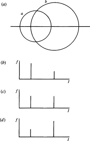
Figure 3.17 Variation in local intensity distribution with position of neighborhood: (a) neighborhood of radius a overlapping a dark circular object of radius b;(b)-(d) intensity distributions I when the separations of the centers are, respectively, less than, equal to, or greater than the distance d for which the object bisects the area of the neighborhood.

Next suppose that the edge is irregular with several “bumps” (i.e., prominences or indentations) within the filter neighborhood. The filter will now tend to average out the bumps and straighten the edge, because it acts in such a way as to form a boundary on which the amounts of dark and light within the neighborhood are equalized (Fig. 3.18). This means that the edge will be locally biased but only by a reduced amount, since the various bumps will tend to pull the final edge in opposite directions. On the other hand, if there is one gross bump within the neighborhood—that is if the curvature has the same sign and is roughly constant at all points on the edge within the filter neighborhood—then all these parts of the edge will act in consort and it will be pulled sideways a significant amount by the filter. Thus, a circular section of the boundary constitutes a worst-case situation, for which the filter produces the largest bias in the position of the edge. It is clearly worth finding the size of the worst-case shift, and for this reason we concentrate our attention on circular objects, in the knowledge that all other shapes will give less serious shifts and distortions.

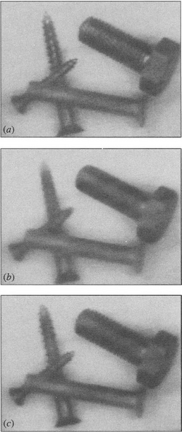
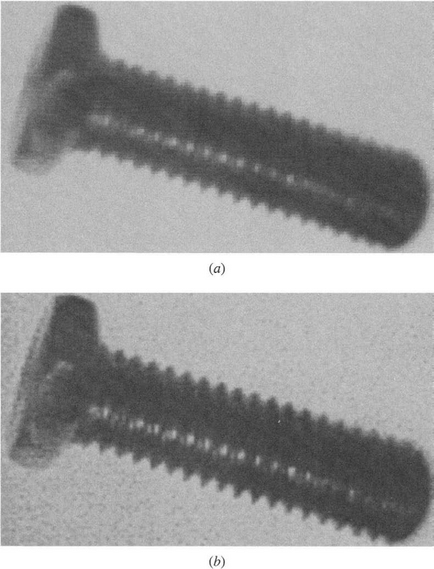
Figure 3.18 Edge smoothing property of the median filter. (a) Original image, (b) median filter smoothing of irregularities, in particular those around the boundaries (notice how the threads on the screws are virtually eliminated, although detail larger in scale than half the filter area is preserved), using a 21-element filter operating within a 5 × 5 neighborhood on a 128 × 128 pixel image of 6-bit gray-scale; (c) effect of a new type of “detail-preserving” filter (see Section 3.8.3).

The worst-case calculation is a matter of elementary geometry: we need to find at what distance d from the center of a circular object (of radius b) the area of a circular neighborhood (of radius a) is bisected by the object boundary.

From Fig. 3.19 the area of the sector of angle 2β is βb² whereas the area of the triangle of angle 2β is b² sin β cos β. Hence, the area of the segment shown shaded is:

Figure 3.19 Geometry for calculating neighborhood and object overlap.

     (3.10)

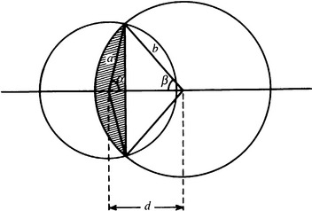
Making a similar calculation of the area A of a circular segment of radius a and angle 2α, we may deduce the area of overlap (Fig. 3.19) between the circular neighborhood of radius a and the circular object of radius b as:

     (3.11)

For a median filter this is equal to πa²/2. Hence:

     (3.12)

where

     (3.13)

and

     (3.14)

To solve this set of equations, we take a given value of d, deduce values of αand β, calculate the value of F, and then adjust the value of d until F = 0. Since d is the modified value of b obtained after filtering, the shift produced by the filtering process is:

     (3.15)

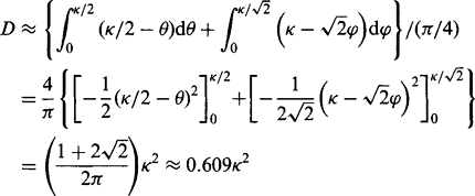
Davies (1989b) has found the results of doing this computation numerically. As expected, D → 0 as b → ∞ or as a → 0. Conversely, the shift becomes very large as a first approaches and then exceeds b. Note, however, that when the object is ignored, being small enough to be regarded as irrelevant noise by the filter: beyond this point it has no effect at all on the final image. The maximum edge shift before the object finally disappears is .

It is instructive to approximate the above equations for the case when edge curvature is small; that is, a << b. Under these conditions, is small, β π/2, and d b. Hence we find:

     (3.16)

After some manipulation, the edge shift D is obtained in the form:

     (3.17)

κ = 1/b being the local curvature. In Chapter 14 this equation is found to be useful for estimating the signals from a median-based corner detector.

3.8.2 Generalization to Gray-scale Images

To extend these results to gray-scale images, first consider the effect of applying a median filter near a smooth step edge in l-D. Here the median filter gives zero shift, since for equal distances from the center to either end of the neighborhood there are equal numbers of higher and lower intensity values and hence equal areas under the corresponding portions of the intensity histogram. This is always valid where the intensity increases monotonically from one end of the neighborhood to the other—a property first pointed out by Gallagher and Wise (1981). (For more recent discussions on related “root” [invariance] properties of signals under median filtering, see Fitch et al., 1985 and Heinonen and Neuvo, 1987.)

Next, it is clear that for 2-D images, the situation is again unchanged in the vicinity of a straight edge, since the situation remains highly symmetrical. Hence, the median filter gives zero shift, as in the binary case.

For curved edges, it again turns out that circular boundaries constitute a worst case that should be considered carefully. However, gray-scale edges are unlike binary edges in that they have finite slope. This means that it is necessary to take account of the exact form of the intensity function within the neighborhood.

When boundaries are roughly circular, contours of constant intensity often appear as in Fig. 3.20. To find how a median filter acts, we merely need to identify the contour of median intensity (in 2-D the median intensity value labels a whole contour), which divides the area of the neighborhood into two equal parts. The geometry of the situation is identical to that already examined in Section 3.8.1. The main difference here is that for every position of the neighborhood, there is a corresponding median contour with its own particular value of shift depending on the curvature. Intriguingly, the formulas already deduced may immediately be applied for calculating the shift for each contour. Figure 3.20 shows an idealized case in which the contours of constant intensity have similar curvature, so that they are all moved inward by similar amounts. This means that, to a first approximation, the edges of the object retain their cross-sectional profile as it becomes smaller.

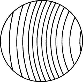
Figure 3.20 Contours of constant intensity on the edge of a large circular object, as seen within a small circular neighborhood.

For gray-scale images the shifts predicted by this theory (with certain additional corrections: see Davies, 1989b) agree with experimental shifts within approximately 10% for a large range of circle sizes in a discrete lattice (see Fig. 3.21). Paradoxically, the agreement is less perfect for binary images, since circles of certain sizes show stability effects (akin to median root behavior). These effects tend to average out for gray-scale images, owing to the presence of many contours of different sizes at different gray levels. Overall, it appears that the edge shifts obtained with median filters are now quite well understood. Figures 3.18 and 3.22 give some indication of the magnitudes of these shifts in practical situations. Note that once image detail such as a small hole or screw thread has been eliminated by a filter, it is not possible to apply any edge shift correction formula to recover it. For larger features, however, such formulas are useful for deducing true edge positions.

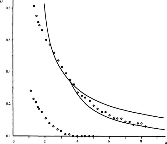
Figure 3.21 Edge shifts for 5 × 5 median filter applied to a gray-scale image. The upper set of plots represents the experimental results, and the upper continuous curve is derived from the theory of Section 3.8.1. The lower continuous curve is derived from a more accurate model (Davies, 1989b). The lower set of plots represents the much reduced shifts obtained with the detail-preserving type of filter (see Section 3.8.3).

Figure 3.22 Circular holes in metal objects before and after filtering: (a) original 128 × 128 pixel image with 6-bit gray-scale; (b)5×5 median-filtered image: the diminution in size of the hole is clearly visible and such distortions would have to be corrected for when taking measurement from real filtered images of this type; (c) result using a detail-preserving filter: some distortions are present although the overall result is much better than in (b).

3.8.3 Shifts Arising with Hybrid Median Filters

Although median filters preserve edges in digital images, they are also known to remove fine image detail such as lines. For example, 3 × 3 median filters remove lines 1 pixel wide, and 5 × 5 median filters remove lines 2 pixels wide. In many applications such as remote sensing and X-ray imaging, this is exceedingly important and efforts have been made to develop filters that overcome the problem. In 1987, Nieminen et al. reported a new class of “detail preserving” filters. These employ linear subfilters whose outputs are combined by median operations. There are a great variety of such filters, employing different subfilter shapes and having the possibility of several layers of median operations. Hence we cannot describe them fully here in the space available. Although these filters are aimed particularly at retention of line detail and are readily understood in this context, they turn out to have some corner preserving properties and to be resistant to the edge shifts that arise when there is a nonzero curvature.

Perhaps the best of the filters in the new class, from the point of view of preserving edge position, is the two-level “bi-directional” linear-median hybrid filter termed 2LH+ (Nieminen et al., 1987). Its operation in a 5 × 5 neighborhood may be illustrated as follows. It employs the subfilters A to I in the 5 × 5 region:

pixels marked as being in the same subfilter having their intensities averaged, and dashed pixels being ignored. Nonlinear filtering then proceeds using two levels of median filtering, with the final center-pixel intensity being taken as:

     (3.18)

Here we ignore the line-preserving properties of this filter and concentrate on its corner-preserving, low-edge-shift characteristics. It is quite easy to see that the 5 × 5 regions

are preserved by this filter, although these examples represent limiting cases that could be disrupted by minor amounts of noise or slight changes of orientation. Thus, the filter seems guaranteed to preserve corners only if the internal angle is greater than 135°. This figure should be compared with the 180° obtained using similar arguments for the normal median filter in 5 × 5 regions such as

Figure 3.21 shows plots obtained with this filter under the same conditions as for the 5 × 5 median filters. It always gives at least a fourfold improvement in edge shift over that for the median filter, and this performance improves with increasing radius of curvature b until there is zero shift for b > 4. (Note that b = 4 is approximately the figure that would be expected from the corner angle of 135^° noted above, within a 5 × 5 neighborhood.) Hence, such detail-preserving filters improve the situation dramatically but do not completely overcome the underlying problem described earlier. In addition, this improvement may not have been obtained without cost, since in some cases the filter seems to insert structure where none exists (Davies, 1989b). The result is to cast some doubt on the usefulness of this type of filter in all possible situations. Nevertheless, its effect on real images appears to be generally very good (see Figs 3.18c and 3.22c).

3.9 Discrete Model of Median Shifts

To produce a discrete model we need to recognize explicitly the positions of the pixels within the chosen neighborhood. We approximate by assuming that the intensity of any pixel is the mean intensity over the whole pixel and is represented by a sample positioned at the center of the pixel. We start by examining the case of a 3 × 3 neighborhood, and proceed by taking the underlying analog intensity variation to have contours of curvature κ, as shown in Fig. 3.20. Following what happened in the continuum case, it will not matter whether the contours of constant intensity are those of a step edge or those of a slowly varying slant edge; it is what happens at the median contour that determines the shift that arises.

The starting point is that zero shift occurs for κ = 0. Next, if κ is even minutely greater than zero, the center pixel will not necessarily be the median pixel. Consider the case when the circular median intensity contour passes close to the center of the neighborhood at a small angle 6 to the positive x-axis (Figs. 3.23 and 3.24a). In that case, the filter will produce a definite shift, whose value is:

Figure 3.23 Geometry for calculation of median shifts on the discrete model. © IEE 1999

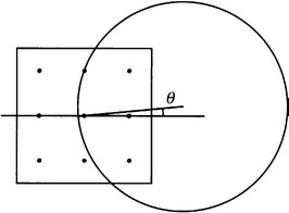
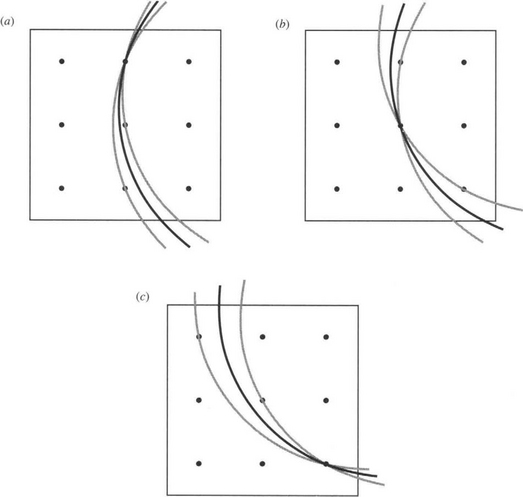
Figure 3.24 Geometry for calculation of median shifts at low κ. These three diagrams show the positions of the median pixels and the ranges of orientations of circular intensity contours for which they apply, (a) for low 9,(b) for intermediate 9, and (c) for high 9.

     (3.19)

where a₀ is the inter-pixel separation—here taken as unity. The first term arises from the following simple result for the geometry of the circle of radius b = 1/κ in Fig. 3.25:

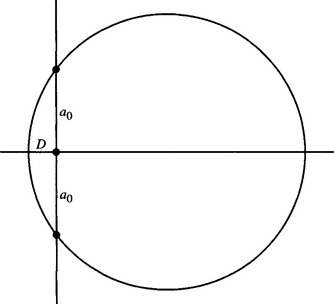
Figure 3.25 Geometry for calculation of shift when the median contour passes through the centers of two pixels.

     (3.20)

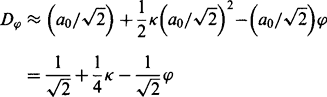
If θ is close to 45°, the shift will have the value:

     (3.21)

where

     (3.22)

and the relevant pixel separation is rather than a₀ (see Fig. 3.24c).

Equations (3.19) and (3.21) show that at the ends of the range 0 ≤ θ ≤ π/4, D_θ varies in proportion to A9. The next problem is understanding what happens when D₉ falls to zero at intermediate values of 9. D₉ remains at zero in this range because the median contour reverts to passing through the central pixel center in the neighborhood (Fig. 3.24b). The resulting approximately piecewise-linear variation in D₉ (Fig. 3.26a) is far from what would be expected on the continuum model. To make a realistic comparison, we must average over all 6. In that case we obtain the result:

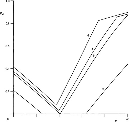
Figure 3.26 Angular variations of 3 × 3 median shifts. (a) Graph showing the situation for κ = 0.4: note that the 6-axis constitutes the middle part of the variation. (b) Graph for higher κ (0.632) when the middle part of the variation just vanishes. (c) Graph for a slightly higher value of κ (0.66). (d) Graph for the highest value of κ (0.7071) for which a valid value of D_θ exists for all 6. Note that (b) is the highest graph for which no change of gradient occurs at high 6. All the graphs presented in this figure are calculated from nonapproximated formulas (Davies, 1999g).

     (3.23)

This shows that D follows a quadratic rather than a linear law at low values of κ, unlike the situation for the continuum model. However, for high values of κ, the variation would be expected to revert to a linear model. This should occur when κ reaches such high values that the range of values of θ for which D_θ = 0 falls to zero. At that stage the whole variation of D_θ with θ should rise bodily as θ increases further (Fig. 3.26). Equating to zero the values of D_θ and D_φ given by the approximate equations (3.19) and (3.21), we deduce that this should happen for values of κ above about . (The accurate value is 0.632—see below.)

Perhaps the most surprising thing is that this hardly happens for a 3 × 3 neighborhood (Figs. 3.26 and 3.27). For the necessary high values of k, the median contour fails to reach all the outermost pixels in the neighborhood and there are orientations for which the contour represents an object that is eliminated entirely by the median filter. Averaging over all 9 is then not meaningful: here we do not consider such cases further.

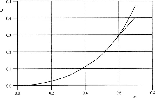
Figure 3.27 Comparisons of 3 × 3 median shifts. The lower solid curve shows the nonapproximated results of the discrete model (Davies, 1999g): the upper solid curve shows the results of experiments on gray-scale circles.

There is one problem with the above interpretation—that for quite high values of κ one other pixel separation than becomes important. This value is (Fig. 3.28c). This leads to the following equation taking over from equation (3.21) at high values of 9:

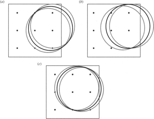
Figure 3.28 Geometry for calculation of median shifts at high κ. These three diagrams show the positions of the median pixels and the ranges of orientations of circular intensity contours for which they apply, (a) for low 6,(b) for intermediate 6, and (c) for high 6.

     (3.24)

To understand in detail when this happens, we should compare Figs. 3.24c and 3.28c. The changeover from one situation to the other occurs when an extreme intensity contour passes through the following three pixel centers: (—1, 0), (0,—1), (1,—1). Such a contour will have a radius , leading to a curvature k 0.632. Curiously, this is the same value as that (noted above) for which the value zero for D₉ drops out of consideration—as is seen by considering Fig. 3.24b, when we find that both extreme intensity contours pass through (1, 0), (0, 0), and (1,—1).

Finally, exact formulas (Davies, 1999g) are used in place of the approximate results of equations (3.19)–equations (3.23) to produce the D₉ graphs in Fig. 3.26 and the average graph in Fig. 3.27.

3.10 Shifts Introduced by Mode Filters

In this section we consider the shifts produced by mode filters in continuous images. As in the cases of median filters, straight edges with symmetrical profiles cannot be shifted by mode filters because of symmetry. We proceed to the two paradigm cases—step edges and slant edges with circular boundaries. Again, the effects of noise will be ignored as we are considering the intrinsic rather than the noise-induced behavior of the mode filtering operation.

The situation for a curved step edge can again be understood by appealing to Fig. 3.17. The result for the mode also has to be identical to that for the median, because the local intensity distribution is exactly symmetrical and bimodal at the point where the median filter switches from a left-hand to a right-hand decision. At that point the mode must give the same result, since the median and the mode are coincident for a symmetrical distribution. Hence, we conclude that the mode also gives a shift of 1/6 κa² for a curved step edge.

Next, we calculate edge shifts in the case where smoothly varying intensity functions exist or—within the confines of a small neighborhood—appear to be smoothly varying. In this case the calculation is especially simple (Davies, 1997c). Using the geometry of Fig. 3.20, we consider the intensity pattern within a circular neighborhood C. Of all the circular intensity contours appearing within C, the one possessing the most frequently occurring intensity, as selected by a mode filter, is the longest. This is the one (M) whose ends are at opposite ends of a diameter of C. To estimate the shift in this case, all we need to do is to calculate the position of M and determine its distance from the center of C. To proceed, we use the well-known formula relating the lengths of parts of intersecting chords of a circle, which gives:³

     (3.25)

Hence:

     (3.26)

That is there is a right shift of the contour, toward the local center of curvature, of 1/2 κa². If we regard this set of contours as forming part of a gray-scale edge profile, then the mode filter shifts the edge through 1/2 κa² toward the center of curvature.

A comment is needed on the marked difference between the cases of step edges and linear intensity profiles. This is all the more interesting as the median filter produces identical shifts of 1/6 κa², for the two profiles (see Table 3.2). Of all the cases listed in Table 3.2, the outstanding one is the large shift for a mode filter operating on a linear intensity profile. Special in this case is that the result relies on a single extreme contour length rather than an average of lengths amounting to an area measure. Hence, it is not surprising that the mode filter gives an exceptionally large shift in this case.

Table 3.2 Candidates for the European Award for Logistics Excellence in 2011

Finally, we note that edge shifts are not avoided merely by choosing an alternative method of neighborhood averaging, but rather that they are intrinsic to the averaging process and can be avoided only by specially designed operators (e.g., see Greenhill and Davies, 1994a).

3.11 Shifts Introduced by Mean and Gaussian Filters

In this section, we consider the shifts produced by mean and Gaussian filters in continuous images. As in the cases of median and mode filters, straight edges with symmetrical profiles cannot be shifted by mean and Gaussian filters, because of symmetry. We again consider the two paradigm cases—step edges and slant edges with circular boundaries. Again, we will ignore the effects of noise because we are considering the intrinsic rather than the noise-induced behavior of the filters.

The situation for a curved step edge can again be understood by appealing to Fig. 3.17. It is identical to that for the median and mode filters, and it follows because of the symmetry of the local intensity distribution at the point where the filter switches from a left-hand to a right-hand decision. At that point the mean filter must give the same result, since all three statistics coincide for a symmetrical distribution. Hence, it also gives a shift of 1/6 κa² for a curved step edge.

In the case of a smoothly varying slant edge, the result for the mean filter has to be calculated by integrating over the area of the neighborhood. The results cannot be obtained by intuitive or simple geometric or intuitive arguments, and here we merely quote the shift for the mean filter as being 1/8 κa².

These considerations complete the entries in Table 3.2. The results for Gaussian filters do not differ substantially from those for mean filters but have to be obtained by integration, taking account of the Gaussian weighting function (Davies, 1991b). All such filters have similar shifting effects because they all incorporate a measure of signal averaging. The shifting effect is not avoided simply by employing a different central-seeking statistic to perform the averaging.

3.12 Shifts Introduced by Rank Order Filters

This section focuses on rank order filters (Bovik et al., 1983), which form a whole family of filters that can be applied to digital images—often in combination with other filters of the family—in order to give a variety of effects (Goetcherian, 1980; Hodgson et al., 1985). Other notable members of the family are max and min filters. Because rank order filters generalize the concept of the median filter, it is relevant to study the types of distortions they produce on straight and curved intensity contours. These filters are of central importance in the design of filters for morphological image analysis and measurement. In addition, they have some advantages when used for this purpose in that they help to suppress noise (Harvey and Marshall, 1995) (though the effect vanishes in the special cases of max and min filters).

Section 3.12.1 examines the reasons underlying the shifts produced by rank order filters and makes calculations of their extent for rectangular neighborhoods. Section 3.12.2 generalizes these results to circular neighborhoods. Section 3.12.3 examines the extent to which the theoretical predictions of the previous sections are borne out in practice by measurements of the shifts produced by 5 × 5 rank order filters on circular discs of varying sizes. It will be taken as axiomatic that the application of rank order filters produces edge shifts on real images (they are well attested in the case of max, min, and median filters). The main question to be answered here is the exact numerical extent of these shifts and how they may be modeled for general rank order filters.

3.12.1 Shifts in Rectangular Neighborhoods

In common with previous work in this area we concentrate here on the ideal noiseless case, in which the filter operates within a small neighborhood, over which the signal is basically a monotonically increasing intensity function in some direction. The most complex intensity variation that will be considered is that in which the intensity contours are curved with curvature k. In spite of this simplified configuration, it will be found that valuable statements can be made about the level of distortion likely to be produced in practice by rank order filters.

Because of the complexity of the calculations that arise in the case of rank order filters, which involve an additional parameter vis-a-vis the median filter, it is worth studying their properties first for the simple case of rectangular neighborhoods (Davies, 2000f). Let us presume that a rank order filter is being applied in a situation in which straight intensity contours are aligned parallel to the short sides of a rectangular neighborhood, which we initially take to be a 1 × n array of pixels (Fig. 3.29). In this case, we can assume without loss of generality that the successive pixels within the neighborhood will have increasing values of intensity. We next take the basic property of the rank order filter as being (effectively or in fact) to construct an intensity histogram of the local intensity distribution and return the value of the rth of the n intensity values within the neighborhood. Thus, the rank order filter selects an intensity that has physical separation B from the lowest intensity pixel of the neighborhood and C from the highest intensity pixel, where:

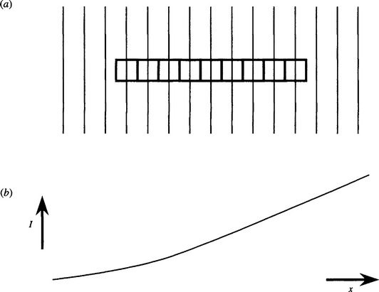
Figure 3.29 Basic situation for a rank-order filter in a rectangular neighborhood. This figure illustrates the problem of applying a rank-order filter within a rectangular neighborhood consisting of a 1 × n array of pixels. The intensity is taken to increase monotonically from left to right, as in (b); the intensity contours in (a) are taken to be parallel to the short sides of the neighborhood.

     (3.27)

     (3.28)

     (3.29)

These definitions emphasize that a rank order filter will in general produce a D-pixel shift, whose value is:

     (3.30)

Before proceeding further, it will be useful to introduce a parameter η that is more symmetrical than r and has value + 1at r = 1and—1at r = n:

     (3.31)

With this notation, which we will use in preference to r throughout the remainder of the chapter, we can write down new formulas for B, C,andD:

     (3.32)

     (3.33)

     (3.34)

The properties of the three paradigm filters are summarized in Table 3.3 in terms of these parameters.

Table 3.3 Properties of the three paradigm filters © RPS [2000]

We now proceed to a continuum model, assuming a large number of pixels in any neighborhood (i.e., n → ∞). The main difference will be that we shall specify distance in terms of the half-length a of the neighborhood rather than in terms of numbers of pixels:

     (3.35)

Next note that this formulation is independent of the width of the neighborhood, as long as the neighborhood is rectangular. We now generalize the situation by taking the neighborhood to be rectangular and of dimensions 2a by 2 (Fig. 3.30).

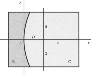
Figure 3.30 Geometry of a rectangular neighborhood with curved intensity contours. Here the neighborhood is a general rectangular neighborhood of dimensions 2a × 2a. Again, the intensity is taken to increase monotonically from left to right; the intensity contours are taken to be parallel and in this case are curved with identical curvature κ. x- and y-axes needed for area calculations are also shown. B and C represent the areas of the two shaded regions on either side of the thick intensity contour.

The next task is to determine the result of a curvature κ = 1/b in the intensity contours. Here we approximate the equation of a circle of radius b, with its diameter on the positive x-axis and passing through the origin, as:

     (3.36)

We can integrate the area under an intensity contour (see Fig. 3.30) as follows:

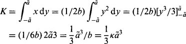     (3.37)

We deduce that the shift D is given by

     (3.38)

     (3.39)

     (3.40)

where

     (3.41)

Hence:

     (3.42)

Equation (3.42) shows that the effects of rank order and of curvature can be calculated and summed separately, the first term being that obtained above for the case of zero curvature and the second term being exactly that calculated for a median filter when the intensity contour is of length 2a~ (the earlier calculation (Davies, 1989b) related to a circular neighborhood). Thus, in principle we merely need to recompute the first term for any appropriate shape of neighborhood. However, there is a complication in that the value of a~ depends on the value of 77 for any neighborhood other than a rectangle.Davies (2000f) has shown how to allow for this complication.

3.12.2 Case of High Curvature

When the curvatures are very high, they may arise from spots that are entirely within the neighborhood, and then there is the possibility that they will be completely eliminated by the rank order filter. (Note that noise points are entirely eliminated by a median filter, which indeed is the prime practical use of that type of filter.) More important, the assumptions of both our model and the exact numerical solution break down when there is no intersection of the circular neighborhood and the intensity contour of radius b = 1/κ. The limiting situation has been studied by Davies (2000f).

Some of the conclusions of this work are quite important. In particular, the result for a median filter is the special case that arises when η= 0, and is in agreement with the calculations of Section 3.8. Next, the max and min filters are also special cases and occur for 77 η =—1 and 1, respectively. In these limiting cases, the shifts are D =—a and a, respectively, the results being independent of κ. This is as might be expected since the value of a~ is zero in each case. Between the max and min filters and the median filter, there is a continuous gradation of performance, with very significant but opposite shifts for the max and min filters, and the two basic effects canceling out for median filters—though the cancellation is only exact for straight contours. The full situation is summarized in Fig. 3.31.

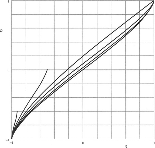
Figure 3.31 Graphs of shift D against rank-order parameter for various κ. This diagram summarizes the operation of rank-order filters, with graphs, bottom to top, respectively, for κ = 0, 0.2/a, 0.5/a,1/a, 2a,5a. Note that graphs for which b< a (κ >1/a) apply for restricted ranges of η and D (see Section 3.12.2). A multiplier of a must be included in the D-values.

3.12.3 Test of the Model in a Discrete Case

Tests of the model were carried out using a truncated 5 × 5 neighborhood with the four corner pixels excluded, in an effort to make the shape a somewhat closer approximation to circular. The resulting rank order filters (with n = 21) were applied to circular discs of various radii. These tests led to the shift variations shown in Fig. 3.32. The uppermost curve represents the theoretical limiting value (Davies, 2000f).

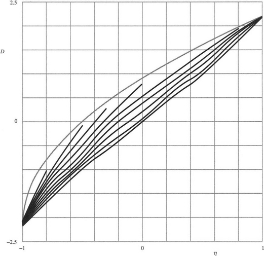
Figure 3.32 Shifts obtained for a typical discrete neighborhood. These shifts were obtained for rank-order filters operating within a truncated 5 × 5 neighborhood when applied to eight discrete circular discs with radii ranging from 10.0 down to 1.25 pixels, the mean curvatures being 0.1 to 0.8 in steps of 0.1. The lowest curve was obtained by averaging the responses from circular discs of radius ±20.0 pixels, with curvatures ±0.05, and to the given scale is indistinguishable from the result that would be obtained with zero curvature. The uppermost curve represents the theoretical limiting value. However, because of the directional effects that occur in the discrete case, the upper limit is actually lower than indicated by this curve (see text).

The variations shown in Fig. 3.32 are very close to what would be expected from Fig. 3.31 (but notice that in Fig. 3.31, a multiplier of a must be included in the D-values, whereas in Fig. 3.32 the D-values are absolute figures for the particular 5 × 5 neighborhood). The upward and downward curl at the ends of the curves—especially that for κ = 0—is not as pronounced in Fig. 3.32 as it is in Fig. 3.31, and the overall shape, while similar, is by no means identical. On the other hand, it is extremely close considering that Fig. 3.31 results from the continuum model, whereas Fig. 3.32 results from a discrete test employing a small neighborhood. It is doubtful whether a more detailed correspondence could be produced without attempting a full discrete model of the shifts. Nevertheless, the limiting values at η = ±1 are observed to be 2.173—well within 1% of the theoretical value 2.174 obtained by calculating the mean distance to the outermost pixels in the 5 × 5 neighborhood (Davies, 2000f).

3.13 The Role of Filters in Industrial Applications of Vision

We have shown how the median filter can successfully remove noise and artifacts such as spots and streaks from images. Unfortunately, many useful features such as fine lines and important points and holes are effectively indistinguishable from spots and streaks. In addition, it has been seen that the median filter “softens” pictures by removing fine detail. It has also been found to clip corners of objects—another generally undesirable trait (but see Chapter 14). Finally, although it does not blur edges, it can still shift them slightly. Shifting of curved edges seems likely to be a general characteristic of noise suppression filters (but see Section 3.8.3).

Such distortions are quite alarming and mitigate against the indiscriminate use of filters. If applied in situations where accurate measurements are to be made on images, particular care must be taken to test whether the data are being biased in any way. Although it is possible to make suitable corrections to the data, it seems a good general policy to employ noise removal filters only where they are absolutely essential for object visibility. The alternative is to employ edge detection and other operators that automatically suppress noise as an integral part of their function. This is the general approach taken in subsequent chapters. Indeed, one of the principles underlined in this book is that algorithms should be “robust” against noise or other artifacts that might upset measurements. There is quite significant scope for the design of robust algorithms, since images contain so much information that it is usually possible to arrange for erroneous information to be ignored.

3.14 Color in Image Filtering

In Chapter 2 we indicated that color often adds to the complexity of image analysis algorithms and could also add to the associated computational costs. From these points of view color might, except for applications such as assessing the ripeness of fruit, be regarded as an irrelevant luxury. Nevertheless, in the field of image processing and image filtering, where good quality images have to be presented to human operators, it is a vital concern. In recent years, much effort has been devoted to the development of effective color filtering algorithms. Here we shall consider mainly median and related impulse noise filtering procedures.

Perhaps the first point to note is that median filtering is defined in terms of sorting operations and is thus undefined in the color domain, which normally contains three dimensions. However, a simple solution is to apply a standard median filter to each of the color channels and then to reassemble the color image. Unfortunately, this approach leads to certain problems, the most obvious one being that of color “bleeding” (Fig. 2.8). This occurs when an impulse noise point appears in just one of the channels and is situated near an edge or other image feature. The case of an impulse noise point near an edge is illustrated in simplified form

original:0 0 0 0 1 0 1 1 1 1 1 1

filtered: ? 0 0 0 0 1 1 1 1 1 1 ?

We see that a three-element median filter eliminates the impulse noise point but at the same time moves the edge toward it. The end result for a color image is that the edge will be tinted with the color of the impulse noise point.

Fortunately, there is a standard solution to this problem. First, note that it is possible to express single-channel median filtering as the minimization of a distance metric, and this metric is trivially extendible to three color channels (or indeed any number of channels). The relevant single channel metric is:

     (3.43)

where d_ij is the distance between sample points i and j in the single-channel (grayscale) space. In the three-color domain the metric is readily extended to:

     (3.44)

where is the generalized distance between sample points i and j, and we typically take the L₂ norm to define the distance measure for three colors:

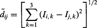     (3.45)

Here I_j, I_j are RGB vectors and I_ik, I_j,k (κI_i,k, I_j,k= 1, 2, 3) are their color components.

Although the resulting vector median filter no longer treats the individual color components separately, it is by no means guaranteed to eliminate color bleeding completely. Like the standard median, it replaces any noisy intensity In, (including color) by the intensity I_j of another pixel that exists in the same window—rather than by an ideal intensity I. Hence, color bleeding is reduced but not eliminated. If indeed there is a confluence of colors at any one point in an image, even in the absence of any impulse noise these sorts of algorithms might become confused and inadvertently introduce small amounts of color bleeding: ultimately, the effect is due to the increased dimensionality of the data, which means that the algorithm has to contend with a greatly increased number of possible outcomes, in spite of being an ad hoc procedure that does not embody specific understanding of images.

Figure 2.8 demonstrates the nature of color bleeding, albeit in the case of mode filtering. This figure shows vector median and vector mode filters to be remarkably free from color bleeding, but the same does not apply to scalar mode filters—for similar reasons to those indicated above for median filters.

3.15 Concluding Remarks

Although this chapter has concentrated on the implementation of noise suppression and image enhancement operators based on the local intensity distribution, it has made certain other points as well. In particular, it has shown the need to make a specification ofthe required imaging process and only then to work out the algorithm design strategy. Not only does this ensure that the algorithm will perform its function effectively, but also it should make it possible to optimize the algorithm for various practical criteria including speed, storage, and other parameters of interest. In addition, this chapter has demonstrated that any undesirable properties of the particular design strategy chosen (such as the inadvertent shifting of edges) should be sought out. Next, it has demonstrated a number of fundamental problems to do with imaging in discrete lattices—not least being problems of statistics that arise with small pixel neighborhoods. Finally, the edge shift work is particularly important in the case of the rather large shifts produced by rank order filters because of their relevance to widely used morphological operators (Chapter 8) where the shifts are turned to advantage.

The next chapter moves on to a particularly vital problem in machine vision—that of segmenting images in order to find where objects are situated. This work builds on what has been learned in the present chapter about edge profiles and how they are “seen” by neighborhood operators.

3.16 Bibliographical and Historical Notes

Much of this chapter has built on a paper by the author (Davies, 1988c) which itself rests on considerable earlier work on Gaussian, median, and other rank order filters (Hodgson et al., 1985; Duin et al., 1986). The edge shifts that occur for median filters are not limited to this type of filter but apply almost equally to mean filters (Davies, 1991b). In addition, other inaccuracies have been found with median filters, and methods have been found to correct them (Davies, 1992f).

The early literature hardly mentions mode filters, presumably because of the difficulty of finding simple mode estimators that are not unduly muddled by noise and that still operate rapidly. Indeed, only one overt reference has been found (Coleman and Andrews, 1979). Other work referred to here is that on decomposing Gaussian and median filters (Narendra, 1978; Wiejak et al., 1985), and the many papers on fast implementation of median filters, both in software and in hardware (e.g., Narendra, 1978; Huang et al., 1979; Ataman et al., 1980; Danielsson, 1981; Davies, 1992a). In particular, there was a strong feeling that VLSI (very large-scale integration) microcircuits would provide the best route for development in this area (Oflazer, 1983; Offen, 1985).

Considerable effort has been devoted to studying the “root” behavior of the median filter, that is, the result of applying median filtering operations until no further change occurs. In fact, most of this work has been carried out on 1-D signals, including cardiac and speech waveforms, rather than on images (Gallagher and Wise, 1981; Fitch et al., 1985; Heinonen and Neuvo, 1987). Root behavior is of interest as it relates to the underlying structure of signals, although its realization involves considerable amounts of processing.

Some of the work on filtering aims to improve on rather than to emulate the median filter. Work of this type includes that of Heinonen and others (Nieminen et al., 1987). See also the neural network approach to this topic discussed in Chapter 25.

Davies (1987e) has reported methods of optimizing linear smoothing filters in small neighborhoods by minimizing the total error in fitting them to a continuous Gaussian function. It turns out that a balance has to be struck between subpixel errors within the neighborhood and errors that arise from the proportion of the distribution that lies outside the neighborhood (Fig. 3.33).

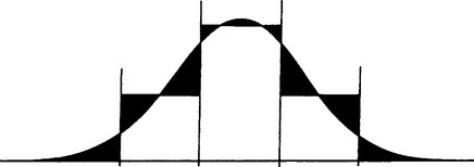
Figure 3.33 Approximating a discrete to a continuous Gaussian. This diagram shows how a balance needs to be struck between subpixel errors and those arising from the truncated part of the function.

More recent work on nonlinear filtering appears in Marshall et al. (1998): see Marshall (2004) for a new design method for weighted order statistic filters.

With the advent of extremely low-cost color frame grabbers on PCs, and the widespread use of digital cameras, digital color images have become ubiquitous, and this has extended to (or even necessitated) much research on color filtering. A convenient summary of work in this area up to 1998 appears in Sangwine and Horne (1998). More recent work on vector (color) filtering includes that of Lukac (2003). Charles and Davies (2003b) describe new distance-weighted median filters and their application to color images. They also extend the author’s earlier mode filter work to color images (Charles and Davies, 2003a, 2004). Davies (2000e) has published a theorem proving that restricting a multichannel (color) filter output to the vector value of one of the input sample points (i.e., from the current window in the image) will increase the inaccuracy present in the final image, for a large proportion of pixels. Since this represents the usual vector median strategy that is employed to minimize color bleeding, the effectiveness of the current generation of color filter algorithms needs to be looked at further.

Davies (1997c, 1998a, 1999g, 2000f) has further analyzed the distortions and edge shifts produced by a range of rank order, mean, and mode filters, and has produced a unified review of the subject (Davies, 2003e). In the case of median filters, it proved possible, and necessary for high accuracy, to produce a discrete model of the situation (Davies, 1998c, 1999d, 1999g, 2003c), rather than extending the continuum model described much earlier (Davies, 1989b).

3.17 Problems

1. Draw up a table showing the number of operations required to implement a median filter in various sizes of the neighborhood. Include in your table (a) results for a straight bubble sort of all n² pixels, (b) results for bubble sorts in separated 1 × n and n × 1 neighborhoods, and (c) results for the histogram method of Section 3.3. Discuss the results, taking account of possible computational overheads.

2. Show how to perform a median filtering operation on a binary image. Also show that if a set of binary images is formed by thresholding a gray-scale image at various levels, and each of these binary images is median filtered, then a gray-scale image can be reconstructed that is a median filtered version of the original grayscale image. Consider to what extent the reduced amount of computation in filtering a binary image compensates for the number of separate thresholded images to be filtered.

3. An “extremum” filter is an image-parallel operation that assigns to every pixel the intensity value of the closer of the two extreme values in its local intensity distribution. Show that it should be possible to use such a filter to enhance images. What would be the disadvantage of such a filter?

4. Under what conditions is a 1-D signal that has been filtered once by a median filter a root signal? What truth is there in the statement that a straight edge in an image is neither shifted nor blurred by a median filter, whatever its cross section?

5. (a) Explain the action of the following median filtering algorithm:

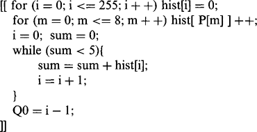
(b) Show how this algorithm can be speeded up (i) by a more efficient histogram clearing technique and (ii) by calculating the minimum intensity in each 3 × 3 window. In each case estimate approximately how much the algorithm will be speeded up.

(c) Explain why a median filter is able to smooth images without introducing blurring.

(d) A 1-D cross section of an image has the following intensity profile:

1 2 1 1 2 3 0 2 2 3 1 1 2 2 9 2 2 8 8 8 7 8 8 7 9 9 9

Apply (i) a three-element median filter and (ii) a five-element median filter to this profile. With the aid of these examples, show that median filters tend to produce “runs” of constant values in 1-D profiles. Show also that under some circumstances an edge in the profile can be shifted by a nearby spike. Give a rule showing when this is likely to occur for an n-element median filter in one dimension.

6. (a) A mode filter is defined as one in which the new pixel intensity at any pixel takes the most probable value in the local intensity distribution of a window placed around that pixel in the original image space. Show for a gray-scale image that a mode filter will, if anything, sharpen the image, while a mean filter will tend to blur the image.

(b) A max filter is one that takes the maximum value of the local intensity distribution in a window around each pixel. Explain what will be seen when a max filter is applied to an image. Consider whether any similar effects are liable to happen when a mode filter is applied to an image.

(c) Explain the purpose of a median filter. Why are 2-D median filters sometimes implemented as two 1-D median filters applied in sequence?

(d) Contrast the behavior of five-element 1-D mean, max, and median filters as applied to the following^†

0 1 1 2 3 2 2 0 2 3 9 3 2 4 4 6 5 6 7 0 8 8 9 1 1 8 9

(e) Work out what would happen if the 1-D median filter were applied many times, starting with this waveform.

7. (a) Determine the effect of applying (i) a 3 × 3 median filter and (ii) a 5 × 5 median filter to the portion of an image shown in Fig. 3.P1.

Figure 3.P1

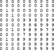
(b) Show that it should be possible to develop a corner detector based on the properties of these median filters. What advantages or disadvantages might result from employing this design strategy?

8. (a) Distinguish between mean and median filtering. Explain why a mean filter would be expected to blur an image, while a median filter would not have this effect. Illustrate your answer by showing what happens in the following 1-D case with a window of size 1 × 3:

1 1 1 1 2 1 1 2 3 4 4 0 4 4 4 5 6 7 6 5 4 3 3

(b) Give a complete median filter algorithm based on histograms and operating within a 3 × 3 window. Explain why it operates relatively slowly.

(c) A computer language has the max(a, b) operation as standard. Show how it may be used to find the maximum intensity within a 3 × 3 window. Show also how it may be used to find the median by successively replacing the maximum values by zeros. If the max(a, b) operation is about the same speed as the a + b operation, determine whether the median can be found any faster by this method.

(d) Discuss whether splitting a 3 × 3 median operation into 1 × 3 and 3 × 1 median operations is likely to be effective in eliminating impulse noise in images. How would the speed of this approach be affected by use of the max(a, b) operation?

9. (a) Determine the result of applying a three-element median filter to the following 1-D signals:

(i) 00000 10111 1111

(ii) 21232122324334

(iii) 11233 45866 7899

(b) What general lessons can be learned from the results? In the first case, consider also the corresponding situation for a gray-scale edge in a 2-D image.

(c) 2-D median filters are sometimes implemented as two 1-D median filters applied in sequence in order to improve the speed of processing. Estimate the gain in speed that could be achieved in this way for (i) a 3 × 3 median filter, (ii) a 7 × 7 median filter, and (iii) in the general case.