
CHAPTER 13 Hole Detection
13.1 Introduction
The last few chapters have been particularly concerned with the direct location of objects from their shapes. Where objects have simple shapes this approach is a viable one, but in more complex situations they may have to be located from their features. In the case of larger objects and assemblies, these features may be components of the very shapes discussed so far. However, two important features have not so far been covered: these are small holes and corners. Corners are dealt with in Chapter 14. Here we will consider the location of small holes: not only can these be used to locate objects and to identify them positively, but also they are important in the task of accurately measuring object dimensions. A later chapter considers carefully how the presence of an object may be deduced once its hole features (or a subset of them) have been found.
We start by considering the template matching approach, which seems a priori the most obvious means of searching an image for small holes. Later sections examine alternative means of carrying out this task. It should be noted that although the chapter is ostensibly about hole location, it is also about methods of searching for such features. In this sense, holes are used as convenient vehicles that allow the relevant principles to be aired.
13.2 The Template Matching Approach
When considering features such as small holes, it is convenient to work with a mental model. We can start by imagining a round, relatively dark region some 1 to 2 pixels in diameter surrounded by a lighter region that is part of some object. The obvious means of detecting such a feature is by template matching. This involves applying a Laplacian type of operator, and in a 3 × 3 neighborhood this may take the form of one of the following convolution masks:
Having applied the convolution, the resulting image is thresholded to indicate regions where holes might be present. Note that if dark holes are regions of negative contrast that are to be located after applying one of the above masks, positions of high negative intensity must be sought. It should be noted in passing that the coefficients in each of the above masks sum to zero so that they are insensitive to varying levels of background illumination.
If the holes in question are larger than 1 to 2 pixels in diameter, the above masks will prove inadequate. Indeed, they will indicate the edges of the holes rather than their centers, and they will also indicate the edges of most objects of similar contrast. In any case, the edges are located with low efficiency since the signal originates from only one-half of the mask. Larger masks are required if larger holes are to be detected efficiently at their centers. For very large holes, the masks that are required are so large that the method becomes impracticable. For example, holes 15 pixels in diameter require masks of size around 22 × 22 pixels. Remembering that these have to be applied at all positions in an image, and assuming that the latter has size 256 × 256 pixels, over 30 million operations are involved. Hence, a better method must be found for locating larger holes. Similar comments clearly apply if any other type of feature is being sought. Indeed, in many cases the problem is then worse, since most such features are not circular, and templates of many different orientations have to be applied in order to locate them effectively.
This problem has been tackled by many workers. Indeed, several powerful general techniques have been developed for this purpose. They include “ordered search” (Nagel and Rosenfeld, 1972), and “coarse-fine” (Rosenfeld and VanderBrug, 1977) and “two-stage” (VanderBrug and Rosenfeld, 1977) template matching. Considerable interest has also been evinced in the basic (Stockman and Agrawala, 1977) and generalized (Ballard, 1981) HT approaches because of their higher inherent efficiency. The next few sections study the lateral histogram technique, which offers significant advantages in certain applications–particularly for corner and round object detection. A later section appraises the situation, taking account of the odd intensity profiles of some holes, and the fact that large holes may be located by the circle detection procedures discussed in Chapter 10.
13.3 The Lateral Histogram Technique
The lateral histogram technique involves projecting an image on two or more axes by summing pixel intensities (see Fig. 13.1) and using the resulting histograms to identify objects in the image. It has been used previously (Pavlidis, 1968; Ogawa and Taniguchi, 1979) as an aid to pattern recognition in binary images, and it has also been applied to the problem of corner detection in gray-scale images (Wu and Rosenfeld, 1983). Here we consider its application to the detection of small round objects and holes, again in gray-scale images.
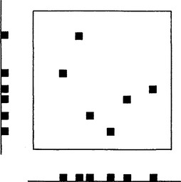
Figure 13.1 The basis of the lateral intensity histogram technique. It is clear that, taken on their own, lateral histograms do not predict object locations uniquely.
The basic technique is inherently attractive in that it requires only about 2N2 pixel operations in an N × N image. However, it turns out that if several similar objects are present in an image, the histograms can be interpreted in a number of ways. Making the method work in practical situations therefore involves finding efficient procedures for resolving ambiguities. It is thus necessary to study the additional computational load these procedures impose. This is done in Sections 13.4-13.5.
13.4 The Removal of Ambiguities in the Lateral Histogram Technique
To resolve the ambiguities that arise with the lateral histogram technique, an obvious strategy is to list all candidate object sites (which arise at the intersections of horizontal and vertical lines corresponding to “hits” in the lateral histograms) and to examine them in turn to check rigorously for the presence of an object (Wu and Rosenfeld, 1983). Basically, the lateral histograms are then used to provide rapid screening of the picture data. All relevant locations are checked subsequently (e.g., by normal template matching) to determine their significance. As a result of this procedure, any artifacts due to random combinations of signals are in the end eliminated. The computational implications of this procedure are assessed in this chapter. Meanwhile, it is worth noting that if the initial level of ambiguity in a particular sequence of images turns out to be high, then it is often possible to rectify the situation by computing the lateral histograms of subimages.
13.4.1 Computational Implications of the Need to Check for Ambiguities
This section shows how many basic computations are required in order to complete the process of object detection and identification. For simplicity, it is assumed that images of size N × N pixels contain p identical objects of size approximately n × n.
First, the number of operations required to obtain each of the lateral intensity histograms is of the order of N2; the number of operations required to perform template matching in each of the two histograms is Nn; and the number of operations required to confirm the presence of an object at each possible object site is around n2. Thus, the total number of operations for the complete algorithm is:
For convenience we shall take a ![]() b
b ![]() c, since this should be a reasonable approximation and sufficiently accurate to give a useful indication of the efficiency of the method.
c, since this should be a reasonable approximation and sufficiently accurate to give a useful indication of the efficiency of the method.
A typical practical case is that of locating holes of diameter 5 pixels in an image of 256 × 256 pixels. If there are 20 holes and a template of size 7 × 7 pixels is required to locate a hole of diameter 5 pixels, then the total number of operations is:
This result should be compared with the result for straight template matching, which is:
Since we have already decided to make the approximation c ![]() a, in the given example it is found that
a, in the given example it is found that
Here the speedup factor is more than 20, so the saving in computational effort is substantial. The checking and 1-D matching procedures reduce the overall saving achieved by the lateral histogram approach very little. The gain in this instance is effectively n2/2. It becomes even more substantial for larger objects (e.g., around 30 for 20 holes of diameter 7 pixels, 50 for 10 holes of diameter 9 pixels, and 400 for 3 holes of diameter 30 pixels).
It is now useful to examine the relative sizes of the terms in equation (13.1). First, the second term is invariably smaller than the first and can essentially be ignored. However, the third term can become so large that it can dominate over the first. In such a situation, it is even possible that the lateral histogram method would require more computational effort than straightforward template matching. Suppose that the computational load of the lateral histogram technique increases to equal that of pure template matching. Then
Since N ![]() 1and n2
1and n2 ![]() 1, it follows that p
1, it follows that p ![]() N. This shows that the lateral histogram technique does not save computation, and using it is not justifiable, if the number of objects approaches N. The danger sign is perhaps when the third term is just equal to the first. This occurs when
N. This shows that the lateral histogram technique does not save computation, and using it is not justifiable, if the number of objects approaches N. The danger sign is perhaps when the third term is just equal to the first. This occurs when
This value of p can be interpreted as the point at which object projections start to overlap and interpretation consequently becomes more difficult. It therefore seems that use of the method should be restricted to cases when p ≤ N / n, so that (1) interpretation is straightforward and (2) a significant saving in computational effort can result. These ideas give a precise indication of when it is profitable to use the subimage method mentioned in Section 13.4. An image should be broken into subimages whenever the image data make N < np. This is discussed in more detail below.
Finally, the lateral histogram method incorporates feedback by virtue of its two-stage mode of operation. This permits it to adapt optimally to variations in the image data, so that it is both rapid and accurate in its task of object location. However, image variability needs to be monitored in order to confirm that operation can take place within the limits indicated above.
13.4.2 Further Detail on the Subimage Method
If an image is broken down into subimages, then the number of objects in each subimage should vary approximately as the square of subimage size. Suppose that the size of a subimage is N × Ñ and that the number of objects it contains is p. Defining
The equation corresponding to equation (13.1) is then:
Multiplying by α2 to obtain a new equation for the whole image, gives:
Thus, the second term is increased while the third is reduced substantially. Differentiating equation (13.11) with respect to a gives:
This is positive at α= 1 for p in the range p < ![]() N/n. Hence, if p is small (typically, p < 4), the subimage method incurs additional computation and should not be used. However, the minimum of Rlat as α varies is shallow, and little is to be gained from using the method until p > N/n, as indicated in Section 13.4.1. Under these circumstances, α should be adjusted so that:
N/n. Hence, if p is small (typically, p < 4), the subimage method incurs additional computation and should not be used. However, the minimum of Rlat as α varies is shallow, and little is to be gained from using the method until p > N/n, as indicated in Section 13.4.1. Under these circumstances, α should be adjusted so that:
Substituting for α in equation (13.11) now gives
The significance of this result is that the third term is limited by the subimage method to one-half the first term and is no longer able to exceed it by a large factor. The second term remains relatively unimportant since it varies as p instead of p2. This means that rarely is there likely to be any penalty from using the subimage method. However, a practical limitation exists, which is now considered.
The practical limitation involves the problem of “edge effects” between subimages. If an object falls on the border between two subimages, then it may escape detection. To overcome this problem, it is necessary to permit subimages to overlap–a factor that will plainly reduce efficiency. The amount by which subimages will have to overlap is equal to the diameter of the objects being detected, since when an object starts to move out of one subimage, it must already be included totally in an adjacent subimage. This means that N must be replaced by Ñ + n in equation (13.10). (N must now be defined by equation (13.8) and is no longer the subimage size.) As a consequence, the additional terms 4Nαn + 4α2 n2 appear in equation (13.11). These dominate over the first term if a ![]() N/2n, i.e. n
N/2n, i.e. n ![]() Ñ/2.
Ñ/2.
Yet there is one way of reducing this problem and getting back substantially to the level indicated by equation (13.16)–namely, by hierarchical addition of rows and columns of pixel intensities while computing the lateral histograms. For example, sub-subimages of some fraction of the size of the subimages may be computed first. These may then be added in appropriate groups. If the size of the subimages is reasonably large (Ñ + n ![]() 1), the final set of summations consumes relatively little computational effort, and equation (13.16) is a realistic approximation.
1), the final set of summations consumes relatively little computational effort, and equation (13.16) is a realistic approximation.
This subsection has shown that when p > N/n, the amount of computational effort needed to locate objects can be kept within reasonable bounds (of order 3N 2) by use of the subimage method. These bounds are remarkably close to those (of order 2N 2) which apply when p ![]() N/n. Bounds of size N2 would, of course, be ideal. It is not expected that significantly different results would apply if the coefficients a, b, c were not exactly equal as assumed above.
N/n. Bounds of size N2 would, of course, be ideal. It is not expected that significantly different results would apply if the coefficients a, b, c were not exactly equal as assumed above.
13.5 Application of the Lateral Histogram Technique for Object Location
We now consider what types of image data can be analyzed conveniently with the aid of lateral histograms. An important feature of the approach is that it is not limited to use in binary images, since all the procedures that are employed (e.g., template matching) are equally applicable to gray-scale images. Another feature of the approach is that objects are identified from their 1-D templates. This means that they may be difficult to locate in the lateral histograms if these are very orientation-dependent. Thus, the method is well adapted to the location of round objects. A great many products, from foodstuffs to machined parts, are almost exactly circular (Davies, 1984c), so the approach is frequently valuable. In addition, many components contain accurately machined circular holes, which can be used to detect the products in which they appear (Chapter 15). Significantly, the method can locate objects whose intensity profiles do not possess well-defined edges (see Fig. 13.2). In such situations the HT method cannot easily be applied because its use requires rapid location and orientation of edges.
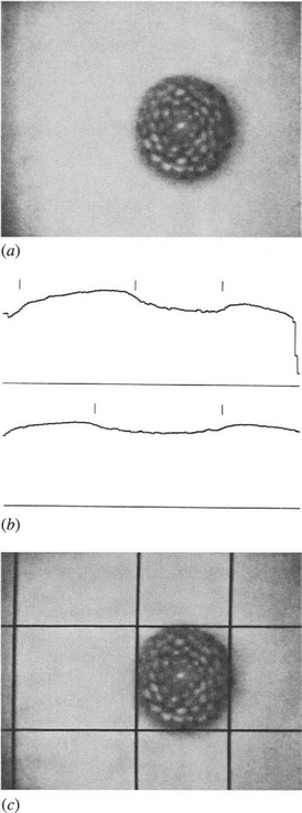
Figure 13.2 (a) Image of a decorative candle that appears as a fairly diffuse object with a fuzzy edge; (b) lateral histograms; (c) edges of the object as detected by differentiating the histograms and locating peaks. The false peak resulting from strongly varying backgrounds is easily eliminated.
Thus, the lateral histogram approach is valuable for the efficient location of (1) small round objects or holes, and (2) objects that are fairly large, round, and somewhat fuzzy or low in contrast. If the number of objects is not excessive, they should be located rapidly and reliably. The author has tested the method on a variety of data from foodstuffs to mechanical parts and has confirmed its value in these applications for images of up to 128 × 128 pixels. For images of these sizes, the subimage method did not have to be used, but for images of 512 × 512 or larger, the subimage method will be required.
Figure 13.3 shows the histograms obtained for images of metal bars containing holes (see Fig. 13.4). All the holes were located by the method, despite their high variability and noise content and despite the rather rudimentary templates used to analyze the histograms (see Fig. 13.5). One or two comments should be made about the initial application of lateral histograms to find candidate hole locations (see Fig. 13.4). First, occasional false positives arose from noise or strong corners (Fig. 13.4a-c,f). Second, on some occasions lateral juxtaposition of holes caused “pulling” and merging of estimated candidate positions (Fig. 13.4b-e). Third, in two cases holes were located in only one histogram (Fig. 13.4e, f). More will be said about this matter in Section 13.5.1. These deficiencies are easily corrected in the final template matching procedure.
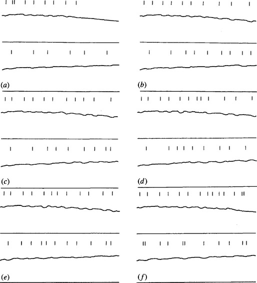
Figure 13.3 Lateral histograms for images of metal bars containing holes for original versions of images in Fig. 13.4.
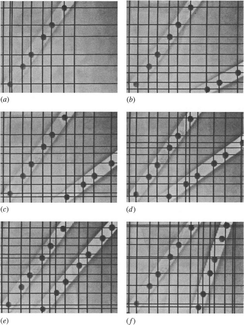
Figure 13.4 Result of applying lateral histograms shown in Fig. 13.3 to find candidate hole positions.
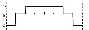
Figure 13.5 Form of the 1-D templates used to locate the hole profiles in the lateral histograms of Fig. 13.3. Greater sophistication was not necessary in this instance.
13.5.1 Limitations of the Approach
When applying lateral histograms for object detection in industrial images, the most serious drawback is that some objects may mask others. Ideally, this problem would not arise, because the intensity patterns of all objects are incorporated additively in the histograms, and any suspicion of an object at a particular location would be checked in detail.
In practice, the most likely masking error arises when the edges of an object are masked by other objects on both sides. (If only one of an object’s edges is so masked, it will almost certainly be detected.) This effect is seen in Fig. 13.4e and 13.4f although in Fig. 13.4f one of the masking objects is a strong corner in the image. The probability of this occurring is quite low. The probability may be estimated by considering the chance of throwing p balls into N boxes, arranged in line, so that three balls fall into any set of three adjacent boxes. Detailed calculations (Davies, 1987g) show that, if the probability of missing an object must be less than 0.01, the maximum number of objects that can be detected in this way is about 20 in a 128 × 128 pixel image–though this number will fall off in the presence of noise. These values are generally in accordance with observations for industrial images.
As already seen from Fig. 13.4, false positives can also arise with the lateral histogram technique. However, since the method involves the use of feedback, false positives are rigorously checked in every case, and the final incidence of false predictions can be no worse than for normal template matching. The number of false positives is strongly related to the amount of noise present in the image; further discussion of this is curtailed inasmuch as the effect is so data-dependent.
13.6 Appraisal of the Hole Detection Problem
Much of this chapter has focused on study of the lateral histogram technique because it is a highly efficient means of locating holes, though not its only application. In this section, we return to a more careful appraisal of methods for hole detection.
At this stage, an obvious question is whether the usual methods for circular object detection can be applied to hole detection. In principle, this is undoubtedly practicable; in many cases, the only change arises because holes have negative contrast. Accordingly, if the HT technique is used, votes will have to be accumulated on moving a distance–R along the direction of the local edge normal.
Small holes, however, are rarely found to have an intensity pattern that matches that of the model introduced in Section 13.2. Figure 13.6 shows some of the possibilities. The basic problem is that it is virtually impossible to make lighting totally diffuse. On the contrary, it usually has significant directionality, so there will be a region of shadow on one side of the hole. Assuming that the holes are infinitely deep but narrow, the region of shadow may well stretch halfway across the width of each hole. If the holes are little more than shallow depressions in the surface, there may be no shadows, but luminous intensity will be graded across each hole. Finally, complications arise because holes are often only a few pixels across, so the arrangements of pixel intensities are unlikely to be smoothly varying. In any case, noise can have a significant effect on the appearance of a hole.
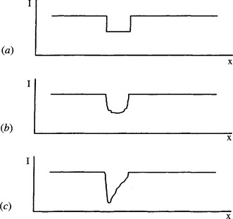
Figure 13.6 (a) Cross-sectional intensity pattern of an idealized hole; (b) a more commonly found case; (c) the effect of the hole being lit obliquely, a significant part of the hole being in shadow.
In summary, four factors can affect the form of a hole in a digitized image: (1) isotropic variations in intensity over the hole region, (2) anisotropic variations in intensity, (3) digitization effects (both spatial and gray-scale), and (4) noise. Since a perfect working model of a hole is unlikely, even in respect of (1), methods for detecting holes need to include a significant amount of averaging to overcome these effects. For example, when an HT circle detector is applied in such cases, for diameters of 10 pixels or less, edge orientation accuracy and edge position accuracy are frequently poor. In addition, the boundary has very few edge points, so little averaging can occur. Hence, peaks in parameter space are ill-defined and the accuracy of center location is poor. (As a percentage measurement it is very poor, while absolutely it may be little better than ±1 pixel.) In contrast, the lateral histogram method incorporates significant averaging and usually arrives at reasonable estimates of hole position. The remaining problem is that factor (2) can result in a systematic bias in estimates of hole position, although it is possible that this can be measured and corrected for.
Finally, it should be observed that the HT approach requires use of an edge detector. If a Sobel operator is employed, the total amount of computation involved will be at least 2 × 8 × N2 = 16N2, many times that required by the lateral histogram method.
Despite these arguments, a hole must at some point become so large that it is better considered as a circle. This point depends particularly on image resolution, but it also varies with the lighting scheme and with the detailed characteristics (shape, smoothness, etc.) of the hole, as indicated above. Hence, the optimum solution is highly data-dependent. Suffice it to say that if holes are smaller than about 16 pixels in diameter, they are probably best detected by the lateral histogram method; if larger than this, they are probably best treated as normal circular objects and detected by an HT method.
Finally, we consider briefly the algorithm of Kelley and Gouin (1984). This algorithm works by finding the midpoints of horizontal and vertical chords of dark areas in an image and locating holes at the center of the resulting cross. Although the method apparently worked adequately on Kelley and Gouin’s data for holes around 12 pixels in diameter, it is liable to fail on less ideal images (e.g., lower contrast or where there are interfering features) since ultimately it relies on the presence of the four edge pixels at the ends of the horizontal and vertical diameters of the holes. Overall, there seems to be no reason to abandon the conclusion that an effective hole-finder needs to incorporate significant averaging, both for general robustness and for accuracy of center location.
13.7 Concluding Remarks
This chapter has aimed to show some of the problems involved in detecting small holes. For all but the smallest holes, template matching is likely to be too computationally intensive. The lateral histogram technique offers a useful solution: it is able to make significant savings in computation since it reduces the dimensionality of the basic search task from two dimensions to one. However, quite large holes are generally best treated as circular objects and detected by an HT technique.
Yet again problems of lighting have arisen, and with them the task of problem specification. Without an accurate problem specification, diagnosis is liable to be inaccurate and algorithm design suboptimal. However, this chapter has been able to show the parameters important in the task of hole detection.
Detection of small holes is a key factor in the location of industrial components. This chapter has shown how this may be achieved with minimal computation using lateral histograms. As with other reduced dimensionality techniques, integrated measures must be employed to avoid ambiguities. In practice, accuracy of hole detection may be limited by lighting problems.
13.8 Bibliographical and Historical Notes
Hole detection is inherently a search problem that would normally involve template matching (correlation). Where template masks are large, some form of speedup is vital and basic methods for achieving this were devised in the 1970s (Nagel and Rosenfeld, 1972; Rosenfeld and VanderBrug, 1977; VanderBrug and Rosenfeld, 1977). At much the same time, it was discovered (Stockman and Agrawala, 1977) that the HT technique (Hough, 1962; Ballard, 1981) is a form of template matching and offers significant savings in computation if edge orientation information is taken into account (Kimme et al., 1975). Lateral intensity histograms were developed for character recognition and later used for corner detection (Pavlidis, 1968; Ogawa and Taniguchi, 1979; Wu and Rosenfeld, 1983). Subsequently, Davies used them for hole detection (1985a, 1987g); Sections 13.3 13.5 embody this work. See also Davies and Barker (1990). Perhaps oddly, the literature gives far greater attention to corner detection than to hole detection (see Chapter 14).
In this chapter holes have been regarded as examples of salient point features that can be used to help locate objects. In principle, they are as suitable as corners for locating industrial components such as brackets and hinges. However, we shall see in Chapter 14 (particularly Section 14.14) that in other applications holes have little part to play–as, for example, when forming correspondences between binocular images of outdoor scenes. In that case “interest” point detectors are needed, and the main characteristics of suitable interest points are that they be distinctive and accurately localizable, not that they approximate to true corners or have the isotropy of holes. For such purposes, the methods of this chapter are not required. This does not represent a failure in any sense–merely the need to find suitable features and detectors to serve the particular purpose to which they will be put (as some would say: “horses for courses”).
13.9 Problems
1. Calculate the bias in the estimated position of a hole if it is illuminated from light at an angle 30° to the vertical and has depth three times its diameter.
2. Find a formula giving the accuracy of a Hough-based hole detector as a function of hole diameter. What other information would be needed to choose between this and other hole detection schemes?
3. Estimate how the basic accuracy of a lateral histogram hole detector varies with the size of the image being used. What limits the accuracy of hole detection with the lateral histogram technique? Is there any possibility of improving it?
4. Work out the probability of missing an object if each of its edges is masked in the histograms between those of two other objects. Hence estimate the maximum number of objects that may be located in an N × N image if the probability of missing an object has to be less than 0.01. (For further details of the problem, see Section 13.5.1.)
5. (a) Explain why it is more efficient to locate an object by its features, instead of as a whole, using template matching. How does locating the object in this way affect the robustness of the process?
(b) Show how feature detection masks may be derived for corner detection, and explain why zero-mean masks are normally used for this purpose. How many masks are needed in this case?
(c) Show that masks such as the following may be used for line segment detection in a 3 × 3 window:
(d) How many masks are needed for this purpose? Why?
(e) Show that line segments may also be detected by small hole detection masks. Explain what is gained by this approach. Show also that holes may be detected by line segment detection masks.
(f) Explain why masks designed for detecting one type of feature may not be quite as effective as tailor-designed masks for detecting other types of feature.