25.1 Introduction

The artificial intelligence community has long been intrigued by the capability of the human mind for apparently effortless perception of complex scenes. Of even greater significance is the fact that perception does not occur as a result of overt algorithms, but rather as a result of hard-wired processes, coupled with extensive training of the neural pathways in the infant brain. The hard-wiring pattern is largely the result of evolution, both of the neurons themselves and of their interconnections, though training and use must have some effect on them too. By and large, however, it is probably correct to say that the overall architecture of the brain is the result of evolution, while its specific perceptual and intellectual capabilities are the result of training. It also seems possible that complex thought processes can themselves move toward solutions on an evolutionary basis, on timescales of milliseconds rather than millennia.

These considerations leave us with two interesting possibilities for constructing artificial intelligent systems: the first involves building or simulating networks of neurons and training them to perform appropriate nontrivial tasks; and the second involves designing algorithms that can search for viable solutions to complex problems by “evolutionary” or “genetic” algorithms (GAs). In this chapter we give only an introductory study of GAs, since their capabilities for handling vision problems are at a preliminary stage. On the other hand, we shall study artificial neural networks (ANNs) more carefully, since they are closely linked to quite old ideas on statistical pattern recognition, and, in addition, they are starting to be used quite widely in vision applications.

Neurons operate in ways that are quite different from those of modern electronic circuits. Electronic circuits may be of two main types—analog and digital—though the digital type is predominant in the present generation of computers. Specifically, waveforms at the outputs of logic gates and flip-flops are strongly synchronized with clock pulses, whereas those at the outputs of biological neurons exhibit “firing” patterns that are asynchronous, often being considered as random pulse streams for which only the frequency of firing carries useful information. Thus, the representation of the information is totally different from that of electronic circuits. Some have argued that the representation used by biological neurons is a vital feature that leads to efficient information processing, and have even built stochastic computing units on this basis. We shall not pursue this line here, for there seems to be no reason why the vagaries of biological evolution should have led to the most efficient representation for artificial information processing; that is, the types of neurons that are suitable for biological systems are not necessarily appropriate for machine vision systems. Nevertheless, in designing machine vision systems, it seems reasonable to take some hints from biological systems on what methodologieght be useful.

This chapter describes ANNs and gives some examples of their application in machine vision, and also gives a brief outline of work on GAs. In considering ANNs, it should be remembered that there are a number of possible architectures with various characteristics, some being appropriate for supervised learning, and others being better adapted for unsupervised learning. We start by studying the perceptron type of classifier designed by Rosenblatt in the 1960s (1962, 1969).

25.2 Artificial Neural Networks

The concept of an ANN that could be useful for pattern recognition started in the 1950s and continued right through the 1960s. For example, Bledsoe and Browning (1959) developed the “n-tuple” type of classifier which involved bitwise recording and lookup of binary feature data, leading to the weightless or logical type of ANN. Although this type of classifier has had some following right through to the present day, it is probably no exaggeration to say that it is Rosenblatt’s “perceptron” (1958, 1962) that has had the greatest influence on the subject.

The simple perceptron is a linear classifier that classifies patterns into two classes. It takes a feature vector x = (x₁, x₂, …, x_N) as its input, and it produces a single scala the classification process being completed by applying a threshold (Heaviside step) function at θ (see Fig. 25.1). The mathematics is simplified by writing–θ as w₀, and taking it to correspond to an input x₀, which is maintained at a constant value of unity. The output of the linear part of the classifier is then written in the form:

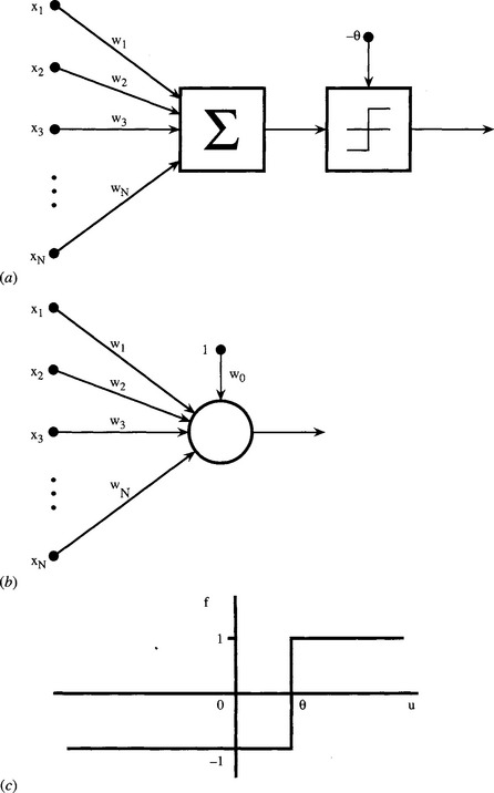
Figure 25.1 Simple perceptron. (a) shows the basic form of a simple perceptron. Input feature values are weighted and summed, and the result fed via a threshold unit to the output connection. (b) gives a convenient shorthand notation for the perceptron; and (c) shows the activation function of the threshold unit.

     (25.1)

and the final output of the classifier is given by:

     (25.2)

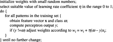
This type of neuron can be trained using a variety of procedures, such as the fixed increment rule given in Fig. 25.2. (The original fixed increment rule used a learning rate coefficient η equal to unity.) The basic concept of this algorithm was to try to improve the overall error rate by moving the linear discriminant plane a fixed distance toward a position where no misclassification would occur—but only doing this when a classification error had occurred:

Figure 25.2 Perceptron fixed increment algorithm.

     (25.3)

     (25.4)

In these equations, the parameter k represents the kth iteration of the classifier, and ω(k) is the class of the kth training pattern. It is important to know whether this training scheme is effective in practice. It is possible to show that, if the algorithm is modified so that its main loop is applied sufficiently many times, and if the feature vectors are linearly separable, then the algorithm will converge on a correct error-free solution.

Unfortunately, most sets of feature vectors are not linearly separable. Thus, it is necessary to find an alternative procedure for adjusting the weights. This is achieved by the Widrow–Hoff delta rule which involves making changes in the weights in proportion to the error δ = ω–d made by the classifier. (Note that the error is calculated before thresholding to determine the actual class: that is, δ is calculated using d rather than f(d).) Thus, we obtain the Widrow–Hoff delta rule in the form:

     (25.5)

There are two important ways in which the Widrow–Hoff rule differs from the fixed increment rule:

These differences underline the revised aim of being able to cope with nonlinearly separable feature data. Figure 25.3 clarifies the situation by appealing to a 2-D case. Figure 25.3(a) shows separable data that are straightforwardly fitted by the fixed increment rule. However, the fixed increment rule is not designed to cope with nonseparable data of the type shown in Fig. 25.3(b) and results in instability during training, as well as inability to arrive at an optimal solution. On the other hand the Widrow-Hoff rule copes satisfactorily with these types of data. An interesting addendum to the case of Fig. 25.3a is that although the fixed increment rule apparently reaches an optimal solution, the rule becomes “complacent” once a zero error situation has occurred, whereas an ideal classifier would arrive at a solution that minimizes the probability of error. The Widrow–Hoff rule goes some way to solving this problem.

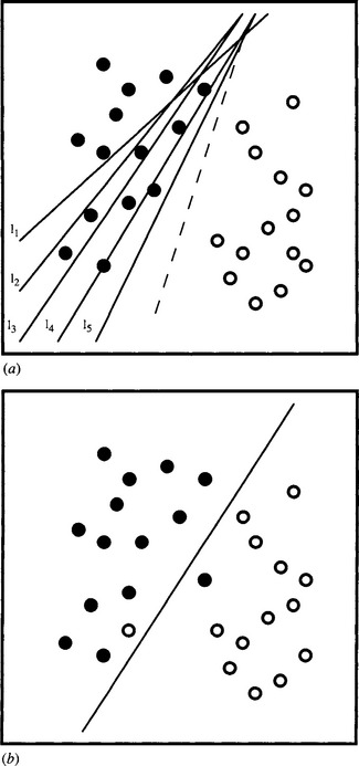
Figure 25.3 Separable and nonseparable data. (a) shows two sets of pattern data. Lines l₁–l₅ indicate possible successive positions of a linear decision surface produced by the fixed increment rule. Note that the fixed increment rule is satisfied by the final position l₅. The dotted line shows the final position that would have been produced by the Widrow–Hoff delta rule. (b) shows the stable position that would be produced by the Widrow–Hoff rule in the case of nonseparable data. In this case, the fixed increment rule would oscillate over a range of positions during training.

So far we have considered what can be achieved by a simple perceptron. Although it is only capable of dichotomizing feature data, a suitably trained array of simple perceptrons—the “single-layer perceptron” of Fig. 25.4—should be able to divide feature space into a large number of subregions bounded (in multidimensional space) by hyperplanes. However, in a multiclass application this approach would require a large number of simple perceptrons—up to for a c-class system. Hence, there is a need to generalize the approach by other means. In particular, multilayer perceptron (MLP) networks (see Fig. 25.5)—which would emulate the neural networks in the brain—seem poised to provide a solution since they should be able to recode the outputs of the first layer of simple perceptrons.

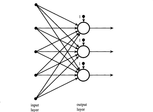
Figure 25.4 Single-layer perceptron. The single-layer perceptron employs a number of simple perceptrons in a single layer. Each output indicates a different class (or region of feature space). In more complex diagrams, the bias units (labeled “1”) are generally omitted for clarity.

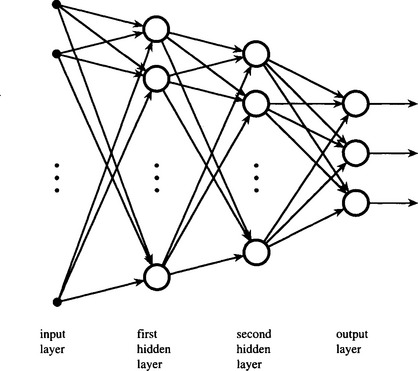
Figure 25.5 Multilayer perceptron. The multilayer perceptron employs several layers of perceptrons. In principle, this topology permits the network to define more complex regions of feature space and thus perform much more precise pattern recognition tasks. Finding systematic means of training the separate layers becomes the vital issue. For clarity, the bias units have been omitted from this and later diagrams.

Rosenblatt himself proposed such networks but was unable to propose general means for training them systematically. In 1969, Minsky and Papert published their famous monograph, and in discussing the MLP raised the spectre of “the monster of vacuous generality”; they drew attention to certain problems that apparently would never be solved using MLPs. For example, diameter-limited perceptrons (those that view only small regions of an image within a restricted diameter) would be unable to measure large-scale connectedness within images. These considerations discouraged effort in this area, and for many years attention was diverted to other areas such as expert systems. It was not until 1986 that Rumelhart et al. were successful in proposing a systematic approach to the training of MLPs. Their solution is known as the backpropagation algorithm.

25.3 The Backpropagation Algorithm

The problem of training an MLP can be simply stated: a general layer of an MLP obtains its feature data from the lower layers and receives its class data from higher layers. Hence, if all the weights in the MLP are potentially changeable, the information reaching a particular layer cannot be relied upon. There is no reason why training a layer in isolation should lead to overall convergence of the MLP toward an ideal classifier (however defined). In addition, it is not evident what the optimal MLP architecture should be. Although it might be thought that this difficulty is rather minor, in fact this is not so. Indeed, this is but one example of the so-called credit assignment problem.¹

One of the main difficulties in predicting the properties of MLPs and hence of training them reliably is the fact that neuron outputs swing suddenly from one state to another as their inputs change by infinitesimal amounts. Hence, we might consider removing the thresholding functions from the lower layers of MLP networks to make them easier to train. Unfortunately, this would result in these layers acting together as larger linear classifiers, with far less discriminatory power than the original classifier. (In the limit we would have a set of linear classifiers, each with a single thresholded output connection, so the overall MLP would act as a single-layer perceptron!)

The key to solving these problems was to modify the perceptrons composing the MLP by giving them a less “hard” activation function than the Heaviside function. As we have seen, a linear activation function would be of little use, but one of “sigmoid” shape, such as the tanh(u) function (Fig. 25.6) is effective and indeed is almost certainly the most widely used of the available functions.²

² We do not here make a marked distinction between symmetrical activation functions and alternatives which are related to them by shifts of axes, though the symmetrical formulation seems preferable as it emphasizes bidirectional functionality. In fact, the tanh(u) function, which ranges from −1 to 1, can be expressed in the form:

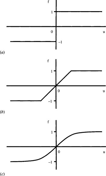
Figure 25.6 Symmetrical activation functions. This figure shows a series of symmetrical activation functions. (a) shows the Heaviside activation function used in the simple perceptron. (b) shows a linear activation function, which is, however, limited by saturation mechanisms. (c) shows a sigmoidal activation function that approximates to the hyperbolic tangent function.

     (25.)

and is thereby closely related to the commonly used function (1 + e^—v)^—1. It can now be deduced that the latter function is symmetrical, though it ranges from 0 to 1 as v goes from–∞ to ∞.

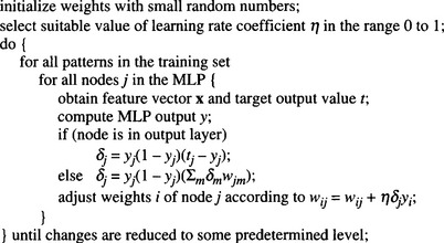
Once these softer activation functions were used, it became possible for each layer of the MLP to “feel” the data more precisely and thus training procedures could be set up on a systematic basis. In particular, the rate of change of the data at each individual neuron could be communicated to other layers, which could then be trained appropriately—though only on an incremental basis. We shall not go through the detailed mathematical procedure, or proof of convergence, beyond stating that it is equivalent to energy minimization and gradient descent on a (generalized) energy surface. Instead, we give an outline of the backpropagation algorithm (see Fig. 25.7). Nevertheless, some notes on the algorithm are in order:

Figure 25.7 The backpropagation algorithm.

When there are many hidden nodes, convergence of the weights can be very slow; this is one disadvantage of MLP networks. Many attempts have been made to speed convergence, and a method that is almost universally used is to add a “momentum” term to the weight update formula, it being assumed that weights will change in a similar manner during iteration k to the change during iteration k–1:

     (25.6)

where α is the momentum factor. Primarily, this technique is intended to prevent networks from becoming stuck at local minima of the energy surface.

25.4 MLP Architectures

The preceding sections gave the motivation for designing an MLP and for finding a suitable training procedure, and then outlined a general MLP architecture and the widely used backpropagation training algorithm. However, having a general solution is only one part of the answer. The next question is how best to adapt the general architecture to specific types of problems. We shall not give a full answer to this question here. However, Lippmann attempted to answer this problem in 1987. He showed that a two-layer (single hidden layer) MLP can implement arbitrary convex decision boundaries, and indicated that a three-layer (two-hidden layer) network is required to implement more complex decision boundaries. It was subsequently found that it should never be necessary to exceed two hidden layers, as a three-layer network can tackle quite general situations if sufficient neurons are used (Cybenko, 1988). Subsequently, Cybenko (1989) and Hornik et al. (1989) showed that a two-layer MLP can approximate any continuous function, though there may sometimes be advantages in using more than two layers.

Although the backpropagation algorithm can train MLPs of any number of layers, in practice, training one layer “through” several others introduces an element of uncertainty that is commonly reflected in increased training times (see Fig. 25.8). Thus, some advantage can be gained from using a minimal number of layers of neurons. In this context, the above findings on the necessary numbers of hidden layers are especially welcome.

Figure 25.8 Learning curve for the multilayer perceptron. Here (a) shows the learning curve for a single-layer perceptron, and (b) shows that for a multilayer perceptron. Note that the multilayer perceptron takes considerable time to get going, since initially each layer receives relatively little useful training information from the other layers. Note also that the lower part of the diagram has been idealized to the case of identical asymptotic error rates—though this situation would seldom occur in practice.

25.5 Overfitting to the Training Data

When training MLPs and many other types of ANN there is a problem of overfitting the network to the training data. One basic aim of statistical pattern recognition is for the learning machine to be able to generalize from the particular set of data it is trained on to other types of data it might meet during testing. In particular, the machine should be able to cope with noise, distortions, and fuzziness in the data, though clearly not to the extent of being able to respond correctly to types of data different from those on which it has been trained. The main points to be made here are (1) that the machine should learn to respond to the underlying population from which the training data have been drawn, and (2) that it must not be so well adapted to the specific training data that it responds less well to other data from the same population. Figure 25.9 shows in a 2-D case both a fairly ideal degree of fit and a situation where every nuance of the set of data has been fitted, thereby achieving a degree of overfit.

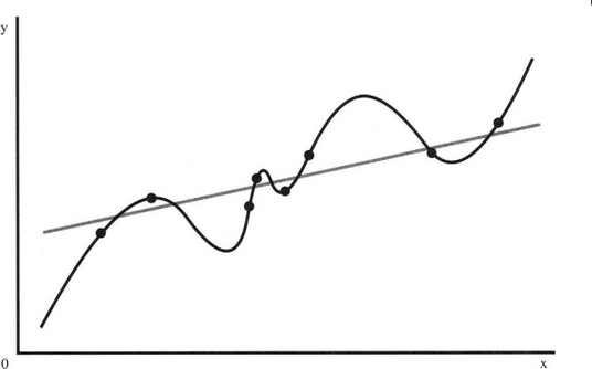
Figure 25.9 Overfitting of data. In this graph, the data points are rather too well fitted by the solid curve, which matches every nuance exactly. Unless there are strong theoretic reasons why the solid curve should be used, the gray line will give a higher confidence level.

Typically, overfitting can arise if the learning machine has more adjustable parameters than are strictly necessary for modeling the training data. With too few parameters, such a situation should not arise. However, if the learning machine has enough parameters to ensure that relevant details of the underlying population are fitted, there may be overmodeling of part of the training set. Thus, the overall recognition performance will deteriorate. Ultimately, the reason for this is that recognition is a delicate balance between capability to discriminate and capability to generalize, and it is most unlikely that any complex learning machine will get the balance right for all the features it has to take account of.

Be this as it may, we need to have some means of preventing overadaptation to the training data. One way of doing so is to curtail the training process before overadaptation can occur.³ This is not difficult, since we merely need to test the system periodically during training to ensure that the point of overadaptation has not been reached. Figure 25.10 shows what happens when testing is carried out simultaneously on a separate dataset. At first, performance on the test data closely matches that on the training data, being slightly superior for the latter because a small degree of overadaptation is already occurring. But after a time, performance starts deteriorating on the test data while that on the training data appears to go on improving. It is at this point that serious overfitting is occurring, and the training process should be curtailed. The aim, then, is to make the whole training process far more rigorous by splitting the original training set into two parts—the first being retained as a normal training set, and the second being called the validation set. Note that the validation set is actually part of the training set in the sense that it is not part of the eventual test set.

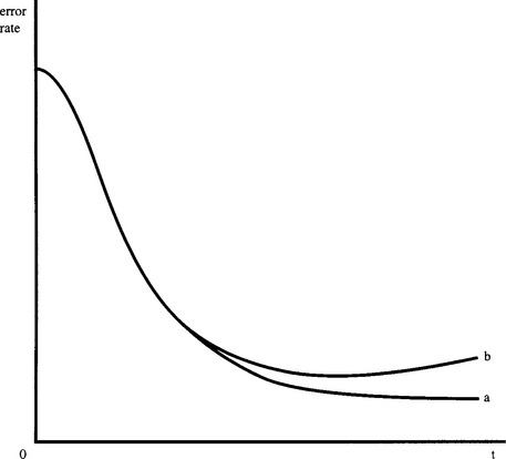
Figure 25.10 Cross-validation tests. This diagram shows the learning curve for a multilayer perceptron (a) when tested on the training data and (b) when tested on a special validation set. (a) tends to go on improving even when overfitting is occurring. However, this situation is detected when (b) starts deteriorating. To offset the effects of noise (not shown on curves (a) and (b)), it is usual to allow 5 to 10% deterioration relative to the minimum in (b).

The process of checking the degree of training by use of a validation set is called cross validation and is vitally important to proper use of an ANN. The training algorithm should include cross validation as a fully integrated part of the whole training schedule. It should not be regarded as an optional extra.

How can overadaptation occur when the training procedure is completely determined by the backpropagation (or other) provably correct algorithms? Overadaptation can occur through several mechanisms. For example, when the training data do not control particular weights closely enough, some can drift to large positive or negative values, while retaining a sufficient degree of cancellation so that no problems appear to arise with the training data. Yet, when test or validation data are employed, the problems become all too clear. The fact that the form of the sigmoid function will permit some nodes to become “saturated out” does not apparently help the situation, for it inactivates parameters and hides certain aspects of the incoming data. Yet it is intrinsic to the MLP architecture and the way it is trained that some nodes are intended to be saturated in order to ignore irrelevant features of the training set. The problem is whether inactivation is inadvertent or designed. The answer probably lies in the quality of the training set and how well it covers the available or potential feature space.

Finally, let us suppose that an MLP is being set up, and it is initially unknown how many hidden layers will be required or how many nodes each layer will have to have. It will also be unknown how many training set patterns will be required or how many training iterations will be required—or what values of the momentum or learning parameters will be appropriate. A quite substantial number of tests will be required to decide all the relevant parameters. There is therefore a definite risk that the final system will be overadapted not only to the training set but also to the validation set. In such circumstances, we need a second validation set that can be used after the whole network has been finalized and final training is being undertaken.

25.6 Optimizing the Network Architecture

In the last section we mentioned that the ANN architecture will have to be optimized. In particular, for an MLP the optimum number of hidden layers and numbers of nodes per layer will have to be decided. The optimal degree of connectivity of the network will also have to be determined (it cannot be assumed that full connectivity is necessarily advantageous—it may be better to have some connections that bypass certain hidden layers).

Broadly, there are two approaches to the optimization of network architectures. In the first, the network is built up slowly node by node. In the second, an overly complex network is built, which is gradually pruned until performance is optimized. This latter approach has the disadvantage of requiring excessive computation until the final architecture is reached. It is therefore tempting to consider only the first of the two options—an approach that would also tend to improve generalization. A number of alternative schemes have been described for optimization that improves generalization. There appears to be no universal best method, and research is still proceeding (e.g., Patel and Davies, 1995).

Instead of dwelling on network generation or pruning aspects of architecture optimization, it is helpful to consider an alternative based on use of GAs. In this approach, various trials are made in a space of possible architectures. To apply GAs to this task, two requirements must be fulfilled. Some means of selecting new or modified candidate architectures is needed; and a suitable fitness function for deciding which architecture is optimal must be chosen. The first requirement fits neatly into the GA formalism if each architecture is defined by a binary codeword that can be modified suitably with a meaningful one-to-one correspondence between codeword and architecture. (This is bound to be possible as each actual connection of a potential completely connected network can be determined by a single bit in the codeword.) In principle, the fitness function could be as simple as the mean square error obtained using the validation set. However, some additional weighting factors designed to minimize the number of nodes and the number of interconnections can also be useful. Although this approach has been tested by a number of workers, the computational requirements are rather high. Hence, GAs are unlikely to be useful for optimizing very large networks.

25.7 Hebbian Learning

In Chapter 24, we found how principal components analysis can help with data representation and dimensionality reduction. Principal components analysis is an especially useful procedure, and it is not surprising that a number of attempts have been made to perform it using different types of ANNs. In particular, Oja (1982) was able to develop a method for determining the principal component corresponding to the largest eigenvalue λ_max using a single neuron with linear weights.

The basic idea is that of Hebbian learning. To understand this process, we must imagine a large network of biological neurons that are firing according to various input stimuli and producing various responses elsewhere in the network. Hebb (1949) considered how a given neuron could learn from the data it receives.⁴ His conclusion was that good pathways should be rewarded so that they become stronger over time; or more precisely, synaptic weights should be strengthened in proportion to the correlation between the firing of pre- and postsynaptic neurons. Here we can visualize the process as “rewarding” the neuron inputs and outputs in proportion to the numbers of input patterns that arrive at them, and modeling this by the equation:⁵

     (25.7)

The problem with this approach is that the weights will grow in an unconstrained manner, and therefore a constraining or normalizing influence is needed. Oja achieved this by adding a weight decay proportional to y²:

     (25.8)

Linsker (1986, 1988) produced an alternative rule based on clipping at certain maximum and minimum values; and Yuille et al. (1989) used a rule that was designed to normalize weight growth according to the magnitude of the overall weight vector w:

     (25.9)

We cannot give a complete justification for these rules here: the only really satisfactory justification requires nontrivial mathematical proofs of convergence. However, these ideas led the way to full determination of principal components by ANNs. Both Oja and Sanger developed such methods, which are quite similar and merit close comparison (Oja, 1982; Sanger, 1989).

First, we consider Oja’s training rule, which applies to a single-layer feedforward linear network with N input nodes, M processing nodes, and transfer functions:

     (25.10)

The rule takes the form:

     (25.11)

This is an extension of the earlier rule for finding the principal component corresponding to λ_max (equation (25.5.2)). In particular, it demands that the M nodes, which are all in the same layer, be connected laterally as shown in Fig. 25.11a, and it is very plausible that if a single node can determine one principal component, then M modes can find M principal components. However, the symmetry of the situation indicates that it is not clear which mode should correspond to the largest eigenvalue and which to any of the others. The situation is less definite than this, and all we can say is that the output vectors span the space of the largest M eigenvalues. The vectors are mutually orthogonal but are not guaranteed to be oriented along the principal axes directions. It should also be noted that the results obtained by the network will vary significantly with the particular data seen during training and their order of presentation. However, the rule is sufficiently good for certain applications such as data compression, since the principal components corresponding to the smallest N–M eigenvalues are systematically eliminated.

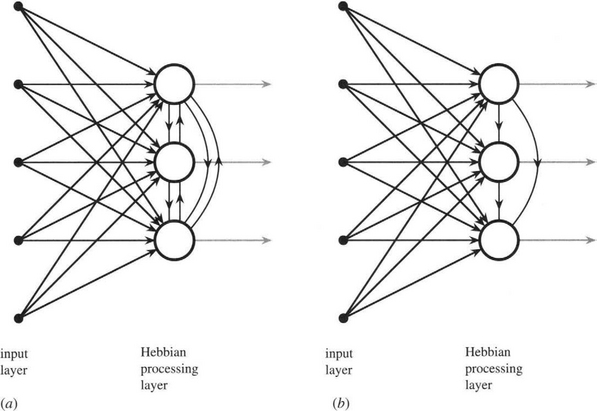
Figure 25.11 Networks employing Hebbian learning. These two networks employ Hebbian learning and evaluate principal components. During training, both networks learn to project the N-dimensional input feature vectors into the space of the M largest principal components. Unlike the Oja network (a), the Sanger network (b) is able to order the output eigenvalues. For clarity, the output connections are shown in gray.

Nevertheless, in many applications it is necessary to force the outputs to correspond to principal components and also to know the order of the eigenvalues. The Sanger network achieves this by making the first node independent of the others; the second dependent only on the first; the third dependent only on the first two; and so on (see Fig. 25.11b). Thus, orthogonality of the principal components is guaranteed, whereas independence is maintained at the right level for each node to be sure of producing a specific principal component. It could be argued that the Sanger network is an M-layer network, though this is arguable as the architecture is obtained from the Oja network by eliminating some of the connections. The Sanger training rule is obtained from the Oja rule by making the upper limit in the summation i rather than N:

     (25.12)

At the end of the computation, the outputs of the M processing nodes contain the eigenvalues, while the weights of the M nodes provide the M eigenvectors. An interesting point arises since the successive outputs of the Sanger network have successively lower importance as the eigenvalues (data variances) decrease. Hence, it is valid and sometimes convenient for images or other output data to be computed and presented with progressively fewer bits for the lower eigenvalues. (This applies especially to real-time hardware implementations of the algorithms.)

It might be questioned whether there is any value in techniques such as principal components analysis being implemented using ANNs when a number of perfectly good conventional methods exist for computing eigenvalues and eigenvectors. When the input vectors are rather large, matrix diagonalization involves significant computation, and ANN approaches can arrive at workable approximations very quickly by iterative application of simple linear nodes that are straightforwardly implemented in hardware. Such considerations are especially important in real-time applications, such as those that frequently occur in automated visual inspection or interpretation of satellite images. It is also possible that the approximations made by ANNs will permit them to include other relevant information, hence leading to increased reliability of data classification, for example, by taking into account higher order correlations (Taylor and Coombes, 1993). Such possibilities will have to be confirmed by future research.

We end this section with a simple alternative approach to the determination of principal components. Like the Oja approach, this method projects the input vectors onto a subspace that is spanned by the first M principal components, discarding only minimal information. In this case the network architecture is a two-layer MLP with N inputs, M hidden nodes, and N output nodes, as shown in Fig. 25.12. The special feature is that the network is trained using the backpropagation algorithm to produce the same outputs as the inputs—a scheme commonly known as self-supervised backpropagation. Note that, unusually, the outputs are taken from the hidden layer. Interestingly, it has been found both experimentally and theoretically that nonlinearity of the neuron activation function is of no help in finding principal components (Cottrell, et al., 1987; Bourland and Kamp, 1988; Baldi and Hornik, 1989).

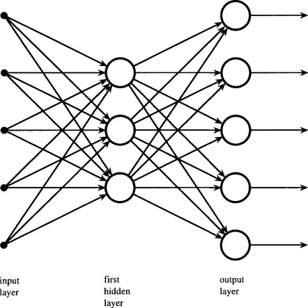
Figure 25.12 Self-supervised backpropagation. This network is a normal two-layer perceptron that is trained by backpropagation so that the output vector tracks the input vector. Once this is achieved, the network can provide information on the M largest principal components. Oddly, this information appears at the outputs of the hidden layer.

25.8 Case Study: Noise Suppression Using ANNs

In what ways can ANNs be useful in applications such as those typical of machine vision? There are three immediate answers to this question. The first is that ANNs are learning machines, and their use should result in greater adaptability than that normally available with conventional algorithms. The second answer is that their concept is that of simple replicable hardware-based computational elements. Hence a parallel machine built using them should in principle be able to operate extremely rapidly, thereby emulating some of the intellectual and perceptual capabilities of the human brain. The third is that their parallel processing capability should lead to greater redundancy and robustness in operation which should again mimic that of the human brain. Although the last two of these possibilities will likely be realized in practice, the position is still not clear, and there is no sign of conventional algorithmic approaches being ousted for these reasons. However, the first point—that of improved adaptability—seems to be at the stage of serious test and practical implementation. It is therefore appropriate to consider it more carefully, in the context of a suitable case study. Here we choose image noise suppression as the vehicle for this study. We use image noise suppression because it is a well researched topic about which a body of relevant theory exists, and any advances made using ANNs should immediately be clear.

As we have seen in Chapter 3, a number of useful conventional approaches are available to image noise suppression. The most widely used, the median filter, is not without its problems, one being that it causes image distortion through the shifting of curved edges. In addition, it has no adjustable parameters other than neighborhood size, and so it cannot be adapted to the different types of noise it might be called upon to eliminate. Indeed, its performance for noise removal is quite limited, as it is largely an ad hoc technique that happens to be best suited to the suppression of impulse noise.

These considerations have prompted a number of researchers to try using ANNs for eliminating image noise (Nightingale and Hutchinson, 1990; Lu and Szeto, 1991; Pham and Bayro-Corrochano, 1992; Yin et al., 1993). Since ANNs are basically recognition tools, they could be used for recognizing noise structures in images, and once a noise structure has been located, it should be possible to replace it by a more appropriate pattern. Greenhill and Davies (1994a, b) have reported a more direct approach in which they trained the ANN how to respond to a variety of input patterns using various example images.

In this work it did not seem appropriate to use an exotic ANN architecture or training method, but rather to test one of the simpler and more widely used forms of ANN. A normal MLP was therefore selected. It was trained using the standard backpropagation algorithm. Preliminary tests were made to find the most appropriate topology for processing the 25 pixel intensities of each 5×5 square neighborhood (the idea being to apply this in turn at all positions in the input images, as with a more conventional filter). The result was a three-layer network with 25 inputs, 25 nodes in the first hidden layer, 5 nodes in the second hidden layer, and one output node, there being 100% connectivity between adjacent layers of the network. All the nodes employed the same sigmoidal transfer function, and a gray-scale output was thus available at the output of the network.

Training was achieved using a normal off-camera image as the low-noise “target” image and a noisy input image obtained by adding artificial noise to the target image. Three experiments were carried out using three different types of noise: (1) impulse noise with intensities 0 and 255; (2) impulse noise with random pixel intensities (taken from a uniform distribution over the range 0 to 255); and (3) Gaussian noise (truncated at 0 and 255). Noise types 1 and 2 were applied to random pixels, whereas noise type 3 was applied to all pixels in the input images. In the experiments, the performances of mean, median, hybrid median (2LH+), and ANN filters were compared, taking particular note of the average absolute deviations in intensity between the output and target images. 3×3 and 5×5 versions of all the filters were used, except that only a 5×5 version of the ANN filter was tried, since it should automatically adapt itself to 3×3 if required by the data seen during training.

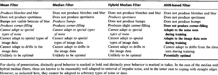
As expected, the mean filters produced gross blurring of the images and “blotchy” behavior as a result of partially averaging impulse noise into the surroundings. Although the median filters eliminated noise effectively, they were found to soften these particular images to an unusual degree (Fig. 25.13), making the beans appear rather unnatural and less like beans than those in the original image. Of the conventional filters, the hybrid median filters gave the best overall performance with these images. However, they allowed a small number of “spotty” noise structures to remain, since these essentially emulated the straight line and corner structures that this type of filter is designed to retain intact (see Section 3.8.3). These particular images seemed prone to another artifact: the fairly straight sides of the beans became “bumpy” after processing by the median filters, this being (predictably) less evident on the images processed by the hybrid median filters. Finally, the median filters gave significant filling in of the corners between the beans, the effect being present but barely discernible after processing by the hybrid median filters. The situation is summarized in Table 25.1.

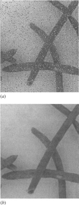
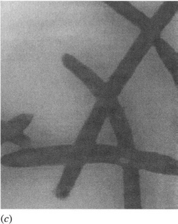
Figure 25.13 Noise suppression by an ANN filter. (a) shows an image with added type 1 impulse noise, (b) shows the effect of suppressing the noise using an appropriately trained ANN filter, and (c) shows the effect of suppressing the noise using a 5×5 median filter. Notice the “softening” effect and the partial filling in of corners in (c), neither of which is apparent in (b).

Table 25.1 Properties of the various filters investigated

In general, the ANN filters⁶ performed better than the conventional filters. First, each was found to perform best with the type of noise it had been trained on and to be more effective than the conventional filters at coping with that particular type of noise. Thus, it exhibited the adaptive capability expected

of it. In addition, the ANN filters produced images without the remanent spottiness, bumpiness, and corner-filling behavior exhibited by the conventional filters.

Nevertheless, the performance of the ANNs was not always exemplary. In one case, an ANN performed less well than a conventional filter when it was tested on an image different from the ones it had been trained on. This must be due to disobeying a basic rule of pattern recognition—namely, that training sets should be fully representative of the classes from which they are drawn (see Chapter 24). However, in this case it could be deemed to have stemmed from the filters being more adapted to the particular type of noise than had been thought possible. Even more surprising was the finding that the training was sensitive not only to the type of noise but also to the types of data in the underlying image. Closer examination of the original images revealed faint vertical camera-induced striations which the ANNs did not remove, but which the median and other filters had eliminated. However, this was because the ANN filters had effectively been “instructed” to keep these striations, since the target images were the original off-camera images, and the input images were produced by adding extra noise to them. Thus, the ANN interpreted the striations as valid image data. A more appropriate training procedure is called for in this problem.

Unfortunately, it is difficult to see how a more appropriate training procedure—or equivalently, a more appropriate set of training images—could be produced. A priori it might have been thought that a median filtered image could be used as a target image. If this were done, however, the ANN would, if anything, exhibit worse performance than the median filter. It would hardly be able to improve on the median filter and adapt effectively to the particular type of noise it is supposed to remove. Such an approach would therefore negate the main aim of using an ANN for noise suppression.

Overall, the results of these experiments are quite significant. They emphasize that ANN-based filters will be limited by the quality of training. It is also useful to notice that any drift in the characteristics of the incoming image data will tend to cause a mismatch between the ANN filter and its training set, so its performance will be liable to deteriorate if this happens. Although this is now apparent for an ANN-based filter, it must also be true to some extent for other more conventional filters, which are by their nature nonadaptable. For example, as noted earlier, a median filter cannot be adapted conveniently and certainly cannot be matched to its data—except by crudely changing the size of its support region. We must now reflect the question back on conventional algorithms: are they general-purpose, or are they adapted to some specific conditions or data (which are in general not known in detail)? For by and large, conventional algorithms stem from the often fortuitous or even opportunistic inspirations of individuals, and their specifications are decided less in advance than in retrospect. Thus, often it is only later that it is found by chance that they have certain undesirable properties that make them unsuitable for certain applications. Table 25.1 summarizes the properties of the various filters examined in these experiments and attempts to highlight their successes and failures.

25.9 Genetic Algorithms

The introduction to this chapter also included GAs as one of the newer biologically inspired methodologies. GAs are now starting to have significant impact on image recognition, and a growing number of papers reflect their use in this area. We start this section by outlining how GAs operate.

Basically, a GA is a procedure that mimics biological systems in allowing solutions (including complete algorithms) to evolve until they become optimally adapted to their situation. The first requirement is a means of generating random solutions. The second requirement is a means of judging the effectiveness of these solutions. Such a means will generally take the form of a “fitness” function, which should be minimized for optimality, though initially very little information will be available on the optimum value. Next, an initial set of solutions is generated, and the fitness function is evaluated for each of them. The initial solutions are likely to be very poor, but the best of them are selected for “mating” and “procreation.” Typically, a pair of solutions is taken, and they are partitioned in some way, normally in a manner that allows corresponding parts to be swapped over (the process is called crossover), thereby creating two combination or “infant” solutions. The infants are then subjected to the same procedures—evaluation of their effectiveness using the fitness function, and placement in an order of merit among the set of available solutions.

From this explanation we see that, if both the infant and the original parent solutions are retained, there will be an increasing population of solutions, those at the top of the list being of increasing effectiveness. The storage of solutions will eventually get out of hand, and the worst solutions will have to be killed off (i.e., erased from memory). However, the population of solutions will continue to improve but possibly at a decreasing rate. If evolution stagnates, further random solutions may have to be created, though another widely used mechanism is to mutate a few existing solutions. This mimics such occurrences as copying errors or radiation damage to genes in biological systems. However, it corresponds to asexual rather than sexual selection, and may well be less effective at improving the system at the required rate. Normally, crossover is taken to be the basic mechanism for evolution in GAs. Although stagnation remains a possibility, the binary cutting and recombination intrinsic to the basic mechanism are extremely powerful and can radically improve the population over a limited number of generations. Thus, any stagnation is often only temporary.

Overall, the approach can arrive at local minima in a suitably chosen solution space, although it may take considerable computation to improve the situation so that a global minimum is reached. Unfortunately, no universal formula has been derived for guaranteeing finding global minima over a limited number of iterations. Each application is bound to be different, and a good many parameters are to be found and operational decisions are to be made. These include:

This approach can be made to operate impressively on such tasks as timetable generation. In such cases, the major decisions to be made are (1) the process of deciding a code so that any solution is expressible as a vector in solution space, and (2) a suitable method for assessing the effectiveness of any solution (i.e., the fitness function). Once these two decisions have been made, the situation becomes that of managing the GA, which involves making the operational decisions outlined above.

GAs are well suited to setting up the weights of ANNs. The GAs essentially perform a coarse search of weight space, finding solutions that are relatively near to minima. Then backpropagation or other procedures can be used to refine the weights and produce optimal solutions. There are good reasons for not having the GAs go all the way to these optimal solutions. Basically, the crossover mechanism is rather brute-force, since binary chopping and recombination are radical procedures that will tend to make significant changes. Thus, in the final stages of convergence, if only one bit is crossed over, there is no certainty that this will produce only a minor change in a solution. Indeed, it is the whole value of a GA that such changes can have rather large effects commensurate with searching the whole of solution space efficiently and quickly.

As stated earlier, GAs are starting to have significant impact on image recognition, and more and more papers that reflect their use in this area are appearing (see Section 25.11). Although algorithms unfortunately run slowly and only infrequently lend themselves to real-time implementation, they have the potential for helping with the design and adaptation of algorithms for which long evolution times are less important. They can therefore help to build masks or other processing structures that will subsequently be used for real-time processing, even if they are not themselves capable of real-time processing (Siedlecki and Sklansky, 1989; Harvey and Marshall, 1994; Katz and Thrift, 1994). Adaptation is currently the weak point of image recognition—not least in the area of automated visual inspection, where automatic setup and adaptation procedures are desperately needed to save programming effort and provide the capability for development in new application areas.

25.10 Concluding Remarks

In the recent past there has been much euphoria and glorification of ANNs. Although this was probably inevitable considering the wilderness years before the backpropagation algorithm became widely known, ANNs are starting to achieve a balanced role in vision and other application areas. In this chapter, space has demanded a concentration on three main topics—MLPs trained using backpropagation, Hebbian networks which can emulate principal components analysis, and GAs. MLPs are almost certainly the most widely used of all the biologically inspired approaches to learning, and inclusion here seems amply justified on the basis of wide utility in vision—with the potential for far wider application in the future. Much the same applies to GAs, although they are at a relatively earlier stage of development and application. In addition, GAs tend to involve considerable amounts of computation, and their eventual role in machine vision is not too clear. All the same, it seems most likely (as indicated in Section 25.9) that they will be more useful for setting up vision algorithms than for carrying out the actual processing in real-time systems.

Returning to ANNs that emulate principal components analysis, we find that it is not clear whether they can yet perform a role that would provide a serious threat to the conventional approach. Important here in determining actual use will be the additional adaptivity provided by the ANN solution, and the possibility that higher order correlations (e.g., Taylor and Coombes, 1993) or nonlinear principal component analysis (e.g., Oja and Karhunen, 1993) will lead to far more powerful procedures that are able to supersede conventional methodologies.

Overall, ANNs now have greater potential for including automatic setup and adaptivity into vision systems than is possible at present, although the resulting systems then become dependent on the precise training set that is employed. Thus, the function of the system designer changes from code writer to code trainer, raising quite different problems. Although this could be regarded as introducing difficulties, it should be noticed that these difficulties are to a large extent already present. For who can write effective code without taking in (i.e., being trained on) a large quantity of visual and other data, all of which will be subject to diurnal, seasonal, or other changes that are normally totally inexplicit? Similarly, for GAs, who can design a fully effective fitness function appropriate to a given application without taking in similar quantities of data?

25.11 Bibliographical and Historical Notes

ANNs have had a checkered history. After a promising start in the 1950s and 1960s, they fell into disrepute (or at least, disregard) during the 1970s following the pronouncements of Minsky and Papert in 1969. They picked up again in the early 1980s and were subjected to an explosion in interest after the announcement of the backpropagation algorithm by Rumelhart et al. in 1986. It was only in the mid-1990s that they started settling into the role of normal tools for vision and other applications. In addition, it should not be forgotten that the backpropagation algorithm was invented several times (Werbos, 1974; Parker, 1985) before its relevance was finally recognized. In parallel with these MLP developments, Oja (1982) led the field with his Hebbian principal components network.

Useful recent general references on ANNs include the volumes by Hertz et al. (1991), Haykin (1999), and Ripley (1996); and the highly useful review article by Hush and Horne (1993). The reader is also referred to two journal special issues (Backer, 1992; Lowe, 1994) for work specifically related to machine vision. In particular, ANNs have been applied to image segmentation by Toulson and Boyce (1992) and Wang et al. (1992); and to object location by Ghosh and Pal (1992), Spirkovska and Reid (1992), and Vaillant et al. (1994). For work on contextual image labeling, see Mackeown et al. (1994). For references related to visual inspection, see Chapter 22. For work on histogram-based thresholding in which the ANN is trained to emulate the maximal likelihood scheme of Chow and Kaneko (1972), see Greenhill and Davies (1995).

GAs were invented in the early 1970s and have only gained wide popularity in the 1990s. A useful early reference is Holland (1975), and a more recent reference is Michalewicz (1992). A short but highly useful review of the subject appears in Srinivas and Patnaik (1994). These references are general and do not refer to vision applications of GAs. Nevertheless, since the late 1980s, GAs have been applied quite regularly to machine vision. For example, they have been used by Siedlecki and Sklansky (1989) for feature selection, and by Harvey and Marshall (1994) and Katz and Thrift (1994) for filter design; by Lutton and Martinez (1994) and Roth and Levine (1994) for detection of geometric primitives in images; by Pal et al. (1994) for optimal image enhancement; by Ankenbrandt et al. (1990) for scene recognition; and by Hill and Taylor (1992) and Bhattacharya and Roysam (1994) for image interpretation tasks. The IEE Colloquium on Genetic Algorithms in Image Processing and Vision (IEE, 1994) presented a number of relevant approaches; see also Gelsema (1994) for a special issue of Pattern Recognition Letters on the subject.

During the early 1990s, papers on artificial neural networks applied to vision were ubiquitous, but by now the situation has settled down. Few see ANNs as being the solution to everything; instead ANNs are taken as alternative means of modeling and estimating, and as such have to compete with conventional, well-documented schemes for performing statistical pattern recognition. Their value lies in their unified approach to feature extraction and selection (even if this necessarily turns into the disadvantage that the statistics are hidden from the user), and their intrinsic capability for finding moderately nonlinear solutions with relative ease. Recent ANN and GA papers include the ANN face detection work of Rowley et al. (1998), among others (Fasel, 2002; Garcia and Delakis, 2002), and the GA object shape matching work of Tsang (2003) and Tsang and Yu (2003). For further information on ANNs and their application to vision, see the books by Bishop (1995), Ripley (1996), and Haykin (1999).