
CHAPTER 8 Mathematical Morphology
8.1 Introduction
In Chapter 2 we met the operations of erosion and dilation, and in Chapter 6 we applied them to the filtering of binary images, showing that with suitable combinations of these operators it is possible to eliminate certain types of objects from images and to locate other objects. These possibilities are not fortuitous, but on the contrary reflect important mathematical properties of shape that are dealt with in the subject known as mathematical morphology. This subject has grown up over the past two or three decades, and over the past few years knowledge in this area has become consolidated and is now understood in considerable depth. This chapter gives some insight into this important area of study. The mathematical nature of the topic mitigated against including the material in the earlier shape analysis chapters, where it might have impeded the flow of the text and at the same time put off less mathematically minded readers. However, these considerations aside, mathematical morphology is not a mere sideline. On the contrary, it is highly important, for it provides a backbone for the whole study of shape, that is capable of unifying techniques as disparate as noise suppression, shape analysis, feature recognition, skeletonization, convex hull formation, and a host of other topics.
Section 8.2 starts the discussion by extending the concepts of expanding and shrinking first encountered in Section 2.2. Section 8.3 then develops the theory of mathematical morphology, arriving at many important results—with emphasis deliberately being placed on understanding of concepts rather than on mathematical rigor. Section 8.4 shows how mathematical morphology is able to cover connectedness aspects of shape. Section 8.5 goes on to show how morphology can be generalized to cope with gray-scale images. Also included in the chapter is a discussion (Section 8.6) of the noise behavior of morphological grouping operations, arriving at a formula explaining the shifts introduced by noise.
8.2 Dilation and Erosion in Binary Images
8.2.1 Dilation and Erosion
As we have seen in Chapter 2, dilation expands objects into the background and is able to eliminate “salt” noise within an object. It can also be used to remove cracks in objects which are less than three pixels in width.
In contrast, erosion shrinks binary picture objects and has the effect of removing “pepper” noise. It also removes thin object “hairs” whose widths are less than 3 pixels.
As we shall see in more detail, erosion is strongly related to dilation in that a dilation acting on the inverted input image acts as an erosion, and vice versa.
8.2.2 Cancellation Effects
An obvious question is whether erosions cancel out dilations, or vice versa. We can easily answer this question. If a dilation has been carried out, salt noise and cracks will have been removed, and once they are gone, erosion cannot bring them back; hence, exact cancellation will not in general occur. Thus, for the set S of object pixels in a general image I, we may write:
equality only occurring for certain specific types of images. (These will lack salt noise, cracks, and fine boundary detail.) Similarly, pepper noise or hairs that are eliminated by erosion will not in general be restored by dilation:
Overall, the most general statements that can be made are:
We may note, however, that large objects will be made 1 pixel larger all around by dilation and will be reduced by 1 pixel all around by erosion. Therefore, a considerable amount of cancellation will normally take place when the two operations are applied in sequence. This means that sequences of erosions and dilations provide a good basis for filtering noise and unwanted detail from images.
8.2.3 Modified Dilation and Erosion Operators
Images sometimes contain structures that are aligned more or less along the image axes, directions; in such cases it is useful to be able to process these structures differently. For example, it might be useful to eliminate fine vertical lines, without altering broad horizontal strips. In that case the following ‘vertical erosion’ operator will be useful:
 (8.5)
(8.5)though it will be necessary to follow it with a compensating dilation operator1 so that horizontal strips are not shortened:
 (8.6)
(8.6)This example demonstrates some of the potential for constructing more powerful types of image filters. To realize these possibilities, we next develop a more general mathematical morphology formalism.
8.3 Mathematical Morphology
8.3.1 Generalized Morphological Dilation
The basis of mathematical morphology is the application of set operations to images and their operators. We start by defining a generalized dilation mask as a set of locations within a 3 × 3 neighborhood. When referred to the center of the neighborhood as origin, each of these locations causes a shift of the image in the direction defined by the vector from the origin to the location. When several shifts are prescribed by a mask, the 1 locations in the various shifted images are combined by a set union operation.
The simplest example of this type is the identity operation which leaves the image unchanged:

(Notice that we leave the 0’s out of this mask, as we are now focusing on the set of elements at the various locations, and set elements are either present or absent.)
The next operation to consider is:

which is a left shift, equivalent to the one discussed in Section 2.2. Combining the two operations into a single mask:

leads to a horizontal thickening of all objects in the image, by combining it with a left-shifted version of itself. An isotropic thickening of all objects is achieved by the operator:

(this is equivalent to the dilation operator discussed in Sections 2.2 and 8.2), while a symmetrical horizontal thickening operation (see Section 8.2.3) is achieved by the mask:

A rule of such operations is that if we want to guarantee that all the original object pixels are included in the output image, then we must include a 1 at the center (origin) of the mask.
Finally, there is no compulsion for all masks to be 3 × 3. Indeed, all but one of those listed above are effectively smaller than 3 × 3, and in more complex cases larger masks could be used. To emphasize this point, and to allow for asymmetrical masks in which the full 3 × 3 neighborhood is not given, we shall shade the origin—as shown in the above cases.
8.3.2 Generalized Morphological Erosion
We now move on to describe erosion in terms of set operations. The definition is somewhat peculiar in that it involves reverse shifts, but the reason for this will become clear as we proceed. Here the masks define directions as before, but in this case we shift the image in the reverse of each of these directions and perform intersection operations to combine the resulting images. For masks with a single element (as for the identity and shift left operators of Section 8.3.1), the intersection operation is improper, and the final result is as for the corresponding dilation operator but with a reverse shift. For more complex cases, the intersection operation results in objects being reduced in size. Thus the mask:

has the effect of stripping away the left sides of objects (the object is moved right and anded with itself). Similarly, the mask:

results in an isotropic stripping operation, and is hence identical to the erosion operation described in Section 8.2.1.
8.3.3 Duality between Dilation and Erosion
We shall write the dilation and erosion operations formally as A ![]() B and A − B, respectively, where A is an image and B is the mask of the relevant operation:
B and A − B, respectively, where A is an image and B is the mask of the relevant operation:
In these equations, Ab indicates a basic shift operation in the direction of element b of B and A_b indicates the reverse shift operation.
We next prove an important theorem relating the dilation and erosion operations:
where Ac represents the complement of A, and Br represents the reflection of B in its origin. We first note that:2
We now have:3
 (8.12)
This completes the proof. The related theorem:
The fact that there are two such closely related theorems, following the related union and intersection definitions of dilation and erosion given above, indicates an important duality between the two operations. Indeed, as stated earlier, erosion of the objects in an image corresponds to dilation of the background, and vice versa. However, the two theorems indicate that this relation is not absolutely trivial, on account of the reflections of the masks required in the two cases. It is perhaps curious that, in contrast with the case of the de Morgan rule for complementation of an intersection:
the effective complementation of the dilating or eroding mask is its reflection rather than its complement per se, while that for the operator is the alternate operator.
8.3.4 Properties of Dilation and Erosion Operators
Dilation and erosion operators have some very important and useful properties. First, note that successive dilations are associative:
whereas successive erosions are not. The corresponding relation for erosions is:
The apparent symmetry between the two operators is more subtle than their simple origins in expanding and shrinking might indicate.
means that the order in which dilations of an image are carried out does not matter, and the same applies to the order in which erosions are carried out:
In addition to the above relations, which use only the morphological operators ![]() and
and ![]() , many more relations involve set operations. In the examples that follow, great care must be exercised to note which particular distributive operations are actually valid:
, many more relations involve set operations. In the examples that follow, great care must be exercised to note which particular distributive operations are actually valid:
In certain other cases, where equality might a priori have been expected, the strongest statements that can be made are typified by the following:
Note that the associative relations show how large dilations and erosions might be factorized so that they can be implemented more efficiently as two smaller dilations and erosions applied in sequence. Similarly, the distributive relations show that a large mask may be split into two separate masks that may then be applied separately and the resulting images ored together to create the same final image. These approaches can be useful for providing efficient implementations, especially in cases where very large masks are involved. For example, we could dilate an image horizontally and vertically by two separate operations, which would then be merged together—as in the following instance:

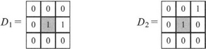
Next, let us consider the importance of the identity operation I, which corresponds to a mask with a single 1 at the central (A0) position:

By way of example, we take equations (8.20) and(8.21) and replace C by I in each of them. If we write the union of B and I as D, so that mask D is bound to contain a central 1 (i.e., D 31), we have:
which is always contained within A:
Operations (such as dilation by a mask containing a central 1) that give outputs guaranteed to contain the inputs are termed extensive, while those (such as erosion by a mask containing a central 1) for which the outputs are guaranteed to be contained by the inputs are termed antiextensive. Extensive operations extend objects, and antiextensive operations contract them, or in either case, leave them unchanged.
Another important type of operation is the increasing type of operation—that is an operation such as union which preserves order in the size of the objects on which it operates. If object F is small enough to be contained within object G, then applying erosions or dilations will not affect the situation, even though the objects change their sizes and shapes considerably. We can write these conditions in the form:
Next, we note that erosion can be used for locating the boundaries of objects in binary images:4
Many practical applications of dilation and erosion follow particularly from using them together, as we shall see later in this chapter.
Finally, we explore why the morphological definition of erosion involves a reflection. The idea is that dilation and erosion are able, under the right circumstances, to cancel each other out. Take the left shift dilation operation and the right shift erosion operation. These are both achieved via the mask:

but in the erosion operation it is applied in its reflected form, thereby producing the right shift required to erode the left edge of any objects. This makes it clear why an operation of the type (A ![]() B)
B)![]() B has a chance of canceling to give A. More specifically, there must be shifts in opposite directions as well as appropriate subtractions produced by anding instead or oring in order for cancellation to be possible. Of course, in many cases the dilation mask will have 180° rotation symmetry, and then the distinction between Br and B will be purely academic.
B has a chance of canceling to give A. More specifically, there must be shifts in opposite directions as well as appropriate subtractions produced by anding instead or oring in order for cancellation to be possible. Of course, in many cases the dilation mask will have 180° rotation symmetry, and then the distinction between Br and B will be purely academic.
8.3.5 Closing and Opening
Dilation and erosion are basic operators from which many others can be derived. Earlier, we were interested in the possibility of an erosion canceling a dilation and vice versa. Hence, it is an obvious step to define two new operators that express the degree of cancellation: the first is called closing since it often has the effect of closing gaps between objects; the other is called opening because it often has the effect of opening gaps (Fig. 8.1). Closing and opening are formally defined by the formulas:

Figure 8.1 Results of morphological operations. (a) shows the original image, (b) the dilated image, (c) the eroded image, (d) the closed image, and (e) the opened image.
Closing is able to eliminate salt noise, narrow cracks or channels, and small holes or concavities.5 Opening is able to eliminate pepper noise, fine hairs, and small protrusions. Thus, these operators are extremely important for practical applications. Furthermore, by subtracting the derived image from the original image, it is possible to locate many sorts of defects, including those cited above as being eliminated by opening and closing: this possibility makes the two operations even more important. For example, we might use the following operation to locate all the fine hairs in an image:
This operator and its dual using opening instead of closing:
are extremely important for defect detection tasks. They are often, respectively, called the white and black top-hat operators.6 (Practical applications of these two operators include location of solder bridges and cracks in printed circuit board tracks.)
Closing and opening have the interesting property that they are idempotent—that is, repeated application of either operation has no further effect. (This property contrasts strongly with what happens when dilation and erosion are applied a number of times.) We can write these results formally as follows:
From a practical point of view, these properties are to be expected, since any hole or crack that has been filled in remains filled in, and there is no point in repeating the operation. Similarly, once a hair or protrusion has been removed, it cannot again be removed without first recreating it. Not quite so obvious is the fact that the combined closing and opening operation is idempotent:
The same applies to the combined opening and closing operation. A simpler result is the following:
which shows that there is no point in opening with the same mask that has already been used for dilation. Essentially, the first dilation produces some effects that are not reversed by the erosion (in the opening operation), and the second dilation then merely reverses the effects of the erosion. The dual of this result is also valid:
Among the most important other properties of closing and opening are the following set containment properties which apply when D 31:
Thus, closing an image will, if anything, increase the sizes of objects, while opening an image will, if anything, make objects smaller, though there are clear limits on how much change closing and opening operations can induce.
Finally, it should be noted that closing and opening are subject to the same duality as for dilation and erosion:
8.3.6 Summary of Basic Morphological Operations
The past few sections have by no means exhausted the properties of the morphological operations dilate, erode, close, and open. However, they have outlined some of their properties and have demonstrated some of the practical results obtained using them. Perhaps the main aim of including the mathematical analysis has been to show that these operations are not ad hoc and that their properties are mathematically provable. Furthermore, the analysis has also indicated (1) how sequences of operations can be devised for a number of eventualities, and (2) how sequences of operations can be analyzed to save computation (for instance) by taking care not to use idempotent operations repeatedly and by breaking masks down into smaller more efficient ones.
Overall, the operations devised here can help to eliminate noise and irrelevant artifacts from images, so as to obtain more accurate recognition of shapes. They can also help to identify defects on objects by locating specific features of interest. In addition, they can perform grouping functions such as locating regions of images where small objects such as seeds may reside (Section 8.6). In general, elimination of artifacts is carried out by operations such as closing and opening, while location of such features is carried out by finding how the results of these operations differ from the original image (cf. equations (8.20) and (8.21)); and locating regions where clusters of small objects occur may be achieved by larger scale closing operations. Care in the choice of scales and mask sizes is of vital importance in the design of complete algorithms for all these tasks. Figures 8.2 and 8.3 illustrate some of these possibilities in the case of a peppercorn image: some of the interest in this image relates to the presence of a twiglet and how it is eliminated from consideration and/or identified.
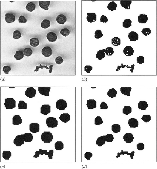
Figure 8.2 Use of the closing operation. (a) shows a peppercorn image, and (b) shows the result of thresholding. (c) shows the result of applying a 3 × 3 dilation operation to the object shapes, and (d) shows the effect of subsequently applying a 3 × 3 erosion operation. The overall effect of the two operations is a ‘closing’ operation. In this case, closing is useful for eliminating the small holes in the objects. This would, for example, be useful for helping to prevent misleading loops from appearing in skeletons. For this picture, extremely large window operations would be required to group peppercorns into regions.
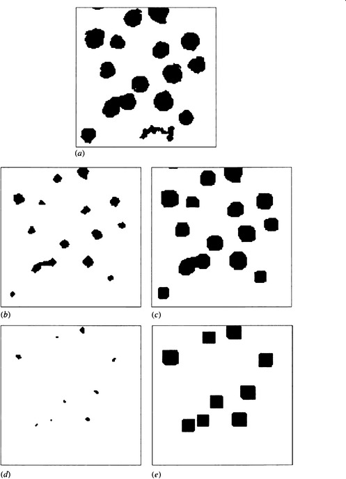
Figure 8.3 Use of the opening operation. (a) shows a thresholded peppercorn image. (b) shows the result of applying a 7 × 7 erosion operation to the object shapes, and (c) shows the effect of subsequently applying a 7 × 7 dilation operation. The overall effect of the two operations is an ‘opening’ operation. In this case, opening is useful for eliminating the twiglet. (d) and (e) show the same respective operations when applied within an 11 × 11 window. Here some size filtering of the peppercorns has been achieved, and all the peppercorns have been separated—thereby helping with subsequent counting and labeling operations.
8.3.7 Hit-and-Miss Transform
We now move on to a transform that can be used to search an image for particular instances of a shape or other characteristic image feature. It is defined by the expression:
The fact that this expression contains an and (intersection) sign would appear to make the description ‘hit-and-miss’ transform more appropriate than the name ‘hit-or-miss’ transform, which is sometimes used.
First, we consider the image analyzing properties of the A ![]() B bracket. Applying B in this way (i.e., using erosion) leads to the location of a set of pixels where the 1’s in the image match the 1’s in the mask. Now notice that applying C to image Ac reveals a set of pixels where the 1’s in C match the 1’s in Ac or the 0’s in A. However, it is usual to take a C mask that does not intersect with B (i.e., (i.e.,B ∩ C =∅︀). This indicates that we are matching a set of 0’s in a more general mask D against the 0’s in A. Thus, D is an augmented form of B containing a specified set of 0’s (corresponding to the 1’s in C) and a specified set of 1’s (corresponding to the 1’s in B). Certain other locations in D contain neither 0’s nor 1’s and can be regarded as ‘don’t care’ elements (which we will mark with an ×). As an example, take the following lower left concave corner locating masks:
B bracket. Applying B in this way (i.e., using erosion) leads to the location of a set of pixels where the 1’s in the image match the 1’s in the mask. Now notice that applying C to image Ac reveals a set of pixels where the 1’s in C match the 1’s in Ac or the 0’s in A. However, it is usual to take a C mask that does not intersect with B (i.e., (i.e.,B ∩ C =∅︀). This indicates that we are matching a set of 0’s in a more general mask D against the 0’s in A. Thus, D is an augmented form of B containing a specified set of 0’s (corresponding to the 1’s in C) and a specified set of 1’s (corresponding to the 1’s in B). Certain other locations in D contain neither 0’s nor 1’s and can be regarded as ‘don’t care’ elements (which we will mark with an ×). As an example, take the following lower left concave corner locating masks:

In reality, this transform is equivalent to a code coincidence detector, with the power to ignore irrelevant pixels. Thus, it searches for instances where specified pixels have the required 0 values and other specified pixels have the required 1 values. When it encounters such a pixel, it marks it with a 1 in the new image space; otherwise it returns a 0. This approach is quite general and can be used to detect a wide variety of local image conditions, including particular features, structures, shapes, or objects. It is by no means restricted to 3 × 3 masks as the above example might indicate. In short, it is a general binary template matching operator. Its power might serve to indicate that erosion is ultimately a more important concept than dilation—at least in its discriminatory, pattern recognition properties.
8.3.8 Template Matching
As indicated in the previous subsection, the hit-and-miss transform is essentially a template matching operator and can be used to search images for characteristic features or structures. However, it needs to be generalized significantly before it can be used for practical feature detection tasks because features may appear in a number of different orientations or guises, and any one of them will have to trigger the detector. To achieve this, we merely need to take the union of the results obtained from the various pairs of masks:
or, equivalently, to take the union of the results obtained from the various D-type masks (see previous subsection).
As an example, we consider how the ends of thin lines may be located. To achieve this, we need eight masks of the following types:
A much simpler algorithm could be used in this case to count the number of neighbors of each pixel and check whether the number is unity. (Alternative approaches can sometimes be highly beneficial in cutting down on excessive computational loads. On the other hand, morphological processing is of value in this general context because of the extreme simplicity of the masks being used for analyzing images.) Further examples of template matching will appear in the following section.
8.4 Connectivity-based Analysis of Images
This chapter has space for just one illustration of the application of morphology to connectedness-based analysis. We have chosen the case of skeletonization and thinning.
8.4.1 Skeletons and Thinning
A widely used thinning algorithm uses eight D-type hit-and-miss transform masks (see Section 8.3.5):
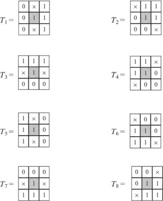
Each of these masks recognizes a particular situation where the central pixel is unnecessary for maintaining connectedness and can be eliminated. (This assumes that the foreground is regarded as 8-connected.) Thus, all pixels can be subjected to the T1 mask and eliminated if the mask matches the neighborhood. Then all pixels can be subjected to the T2 mask and eliminated if appropriate; and so on until upon repeating with all the masks there is no change in the output image (see Chapter 6 for a full description of the process).
Although this particular procedure is guaranteed not to disconnect objects, it does not terminate the skeleton location procedure, as there remain a number of locations where pixels can be removed without disconnecting the skeleton. The advantage of the eight masks given here is that they are very simple and produce fast convergence toward the skeleton. Their disadvantage is that a final stage of processing is required to complete the process. (For example, one of the crossing-number-based methods of Chapter 6 may be used for this purpose, but we do not pursue the matter further here.)
8.5 Gray-scale Processing
The generalization of morphology to gray-scale images can be achieved in a number of ways. A particularly simple approach is to employ ‘flat’ structuring elements. These perform morphological processing in the same way for each of the gray levels, acting as if the shapes at each level were separate, independent binary images. If dilation is carried out in this way, the result turns out to be identical to the effect of applying an intensity maximum operation of the same shape. That is, we replace set inclusion by a magnitude comparison. Needless to say, this is mathematically identical in action for a normal binary image, but when applied to a gray-scale image it neatly generalizes the dilation concept. Similarly, erosion can be carried out by applying an intensity minimum structuring element of the same shape as the original binary structuring element. This discussion assumes that we focus on light objects against dark backgrounds.7 These will be dilated when the maximum intensity operation is applied, and they will be eroded when the minimum intensity operation is applied. We could of course reverse the convention, depending on what type of objects we are concentrating on at any moment, or in any application. We can summarize the situation as follows:
Other more complex gray-scale analogs of dilation and erosion take the form of 3-D structuring elements whose output at any gray level depends not just on the shape of the image at that gray level but also on the shapes at a number of nearly gray levels. Although such ‘nonflat’ structuring elements are useful, for a good many applications they are not necessary, for flat structuring elements already embody considerable generalization relative to the binary case.
Next we consider how edge detection is carried out using grey-scale morphology.
8.5.1 Morphological Edge Enhancement
In Section 2.2.2 we showed how edge detection could be carried out in binary images. We defined edge detection asymmetrically, in the sense that the edge was the part of the object that was next to the background. This definition was useful because including the part of the background next to the object would merely have served to make the boundary wider and less precise. However, edge detection in gray-scale images does not need to embody such an asymmetry8 because it starts by performing edge enhancement and then carrying out a thresholding type of operation—the width being controlled largely by the manner of thresholding and by whether nonmaximum suppression or other factors are brought to bear. Here we start by formulating the original binary edge detector in morphological form; then we make it more symmetrical; finally, we generalize it to gray-scale operation.
The original binary edge detector may be written in the form (cf. equation (8.31)):
Making it symmetrical merely involves adding the background edge ((A ![]() B)–A):
B)–A):
To convert to gray-scale operation involves employing maximum and minimum operations in place of dilation and erosion. In this case we are concentrating on intensity per se, and so these respective assignments of dilation and erosion are used. (The alternate arrangement would result in negative edge contrast.) Thus, here we use equations (8.47) and (8.48) to define dilation and erosion for gray-scale processing, so equation (8.50) already represents morphological edge enhancement for grey-scale images. The argument G is often called the morphological gradient of an image (Fig. 8.4). Notice that it is not accompanied by an accurate edge orientation value, though approximate orientations can, of course, be computed by determining which part of the structuring element gives rise to the maximum signal.
8.5.2 Further Remarks on the Generalization to Gray-scale Processing
In the previous subsection, we found that reinterpreting equation (8.50) permitted edge detection to be generalized immediately from binary to gray-scale. That this is so is a consequence of the extremely powerful umbra homomorphism theorem. This starts with the knowledge that intensityI is a single-valued function of position within the image. This means that it represents a surface in a 3-D (grayscale) space. However, as we have seen, it is useful to take into account the individual gray levels. In particular, we note that the set of pixels of gray level gi is a subset of the set of pixels of gray level gi_1, where gi > gi_ 1. The important step forward is to interpret the 3-D volume containing all these gray levels under the intensity surface as constituting an umbra—a 3-D shadow region for the relevant part of the surface. We write the umbra volume of I as U(I), and clearly we also have I = T(U(I)), where the operator T(-) recalculates the top surface.
The umbra homomorphism theorem then states that a dilation has to be defined and interpreted as an operation on the umbras:
To find the relevant intensity function, we merely need to apply the top-surface operator to the umbra:
A similar statement applies for erosion.
The next step is to note that the generalization from binary to gray-scale dilation using flat structuring elements involved applying a maximum operation in place of a set union operation. The operation can, for the simple case of a 1-D image, be rewritten in the form:
where K(z) takes values 0 or 1 only, and x—z, z must lie within the domains of I and K. However, another vital step is now to notice that this form generalizes to nonbinary K(z), whose values can, for example, be the integer gray-level values. This makes the dilation operation considerably more powerful, yielding the nonflat structuring element concept—which will also work for 2-D images with full grey-scale.
Working out the responses of this sort of operation can be tedious, but it is susceptible to a neat geometric interpretation. If the function K(z) is inverted and turned into a template, this may be run over the image I(x) in such a way as to remain just in contact with it. Thus, the origin of the inverted template will trace out the top surface of the dilated image. The process is depicted in Fig. 8.5 for the case of a triangular structuring element in a 1-D image.

Figure 8.5 Dilation of 1-D grey-scale image by triangular structuring element. (a) shows the structuring element, with the vertical line at the bottom indicating the origin of coordinates. (b) shows the original image (continuous black line), several instances of the inverted structuring element being applied, and the output image (continuous gray line). This geometric construction automatically takes account of the maximum operation in equation (8.53). Note that as no part of the structuring element is below the origin in (a), the output intensity is increased at every point in the image.
Similar relations apply for erosion, closing, opening, and a variety of set functions. This means that the standard binary morphological relations, equations (8.15)–(8.23), apply for gray-scale images as well as for binary images. Furthermore, the dilation-erosion and closing-opening dualities (equations (8.9), (8.13), (8.43), (8.44)) also apply for gray-scale images. These are extremely powerful results and allow one to apply morphological concepts in an intuitive manner. In that case, the practically important factor devolves into choosing the right gray-scale structuring element for the application.
Another interesting factor is the possibility of using morphological operations instead of convolutions in many places where convolution is employed throughout image analysis. We have already seen how edge enhancement and detection can be performed using morphology in place of convolution. In addition, noise suppression by Gaussian smoothing can be replaced by opening and closing operations. However, it must always be borne in mind that convolutions are linear operations and are thereby grossly restricted, whereas morphological operations are highly nonlinear, their very structure embodying multiple if statements, so that outward appearances of similarity are bound to hide deep differences of operation, effectiveness, and applicability. Consider, for example, the optimality of the mean filter for suppressing Gaussian noise, and the optimality of the median filter (a morphological operator) for eliminating impulse noise.
One example is worth including here. When edge enhancement is performed, prior to edge detection, it is possible to show that when both a differential gradient (e.g., Sobel) operator and a morphological gradient operator are applied to a noise-free image with a steady intensity gradient, the results will be identical, within a constant factor. However, if one impulse noise pixel arises, the maximum or minimum operations of the morphological gradient operator will select this value in calculating the gradient, whereas the differential gradient operator will average its effect over the window, giving significantly less error.
Space prevents gray-scale morphological processing from being considered in more detail here; see, for example, Haralick and Shapiro (1992) and Soille (2003).
8.6 Effect of Noise on Morphological Grouping Operations
Texture analysis is an important area of machine vision and is relevant not only for segmenting one region of an image from another (as in many remote sensing applications), but also for characterizing regions absolutely—as is necessary when performing surface inspection (for example, when assessing the paint finish on automobiles). Many methods have been employed for texture analysis. These range from the widely used gray-level co-occurrence matrix approach to Law’s texture energy approach, and from use of Markov random fields to fractal modeling (Chapter 26).
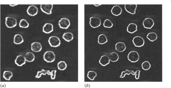
Some approaches involve even less computation and are applicable when the textures are particularly simple and the shapes of the basic texture elements are not especially critical. For example, if it is required to locate regions containing small objects, simple morphological operations applied to thresholded versions of the image are often appropriate (Fig. 8.6) (Haralick and Shapiro, 1992; Bangham and Marshall, 1998). Such approaches can be used for locating regions containing seeds, grains, nails, sand, or other materials, either for assessing the overall quantity or spread or for determining whether some regions have not yet been covered. The basic operation to be applied is the dilation operation, which combines the individual particles into fully connected regions. This method is suitable not only for connecting individual particles but also for separating regions containing high and low densities of such particles. The expansion characteristic of the dilation operation can be largely canceled by a subsequent erosion operation, using the same morphological kernel. Indeed, if the particles are always convex and well separated, the erosion should exactly cancel the dilation, though in general the combined closing operation is not a null operation, and this is relied upon in the above connecting operation.

Figure 8.6 Idealized grouping of small objects into regions, such as might be attempted using closing operations.
Closing operations have been applied to images of cereal grains containing dark rodent droppings in order to consolidate the droppings (which contain significant speckle—and therefore holes when the images are thresholded) and thus to make them more readily recognizable from their shapes (Davies et al., 1998a). However, the result was rather unsatisfactory as dark patches on the grains tend to combine with the dark droppings; this has the effect of distorting the shapes and also makes the objects larger. This problem was partially overcome by a subsequent erosion operation, so that the overall procedure is dilate + erode + erode.
Originally, adding this final operation seemed to be an ad hoc procedure, but on analysis it was found that the size increase actually applies quite generally when segmentation of textures containing different densities of particles is carried out. It is this general effect that we now consider.
8.6.1 Detailed Analysis
Let us take two regions containing small particles with occurrence densities p1, p2, where p1 > p2. In region 1 the mean distance between particles will be d1, and in region 2 the mean distance will be d2, where d1 < d2. If we dilate using a kernel of radius a, where d1 < 2a< d2, this will tend to connect the particles in region 1 but should leave the particles in region 2 separate. To ensure connecting the particles in region 1, we can make 2a larger than (1/2)(d1 + d2), but this may risk connecting the particles in region 2. (The risk will be reduced when the subsequent erosion operation is taken into account.) Selecting an optimum value of a depends not only on the mean distances d1, d2 but also on their distributions. Space prevents us from entering into a detailed discussion of this subject; we merely assume that a suitable selection of a is made and that it is effective. The problem that is tackled here is whether the size of the final regions matches the a priori desired segmentation, that is, whether any size distortion takes place. We start by taking this to be an essentially 1-D problem, which can be modeled as in Fig. 8.7. (The 1-D particle densities will now be given an x suffix.)
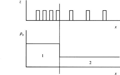
Figure 8.7 1-D particle distribution. z indicates the presence of a particle, and px shows the densities in the two regions.
Suppose first that p2x = 0. Then in region 2 the initial dilation will be counteracted exactly (in 1-D) by the subsequent erosion. Next take p2x > 0: when dilation occurs, a number of particles in region 2 will be enveloped, and the erosion process will not exactly reverse the dilation. If a particle in region 2 is within 2a of an outermost particle in region 1, they will merge and will remain merged when erosion occurs. The probability P that this will happen is the integral over a distance 2a of the probability density for particles in region 2. In addition, when the particles are well separated, we can take the probability density as being equal to the mean particle density p2x. Hence:
If such an event occurs, then region 1 will be expanded by amounts ranging from a to 3a, or 0 to 2a after erosion, though these figures must be increased by b for particles of width b. Thus, the mean increase in size of region 1 after dilation + erosion is 2ap2x × (a + b), where we have assumed that the particle density in region 2 remains uniform right up to region 1.
Next we consider what additional erosion operation will be necessary to cancel this increase in size. We just make the radius a1-D of the erosion kernel equal to the increase in size:
Finally, we must recognize that the required process is 2-D rather than 1-D, and we take y to be the lateral axis, normal to the original (1-D) x-axis. For simplicity we assume that the dilated particles in region 2 are separated laterally and are not touching or overlapping (Fig. 8.8). As a result, the change of size of region 1 given by equation (8.55) will be diluted relative to the 1-D case by the reduced density along the direction (y) of the border between the two regions; that is, we must multiply the right-hand side of equation (8.55) by bp2y. We now obtain the relevant 2-D equation:

Figure 8.8 Model of the incidence of particles in two regions. Region 2 (on the right) has sufficiently low density that the dilated particles will not touch or overlap.
where we have finally reverted to the appropriate 2-D area particle density p2.
For low values of p2 an additional erosion will not be required, whereas for high values of p2 substantial erosion will be necessary, particularly if b is comparable to or larger than a. If a2-D< 1, it will be difficult to provide an accurate correction by applying an erosion operation, and all that can be done is to bear in mind that any measurements made from the image will require correction. (Note that if, as often happens, a ![]() 1, ã2-D could well be at least 1.)
1, ã2-D could well be at least 1.)
8.6.2 Discussion
The work described earlier (Davies, 2000c) was motivated by analysis of cereal grain images containing rodent droppings, which had to be consolidated by dilation operations to eliminate speckle, followed by erosion operations to restore size.9 It has been found that if the background contains a low density of small particles that tend, upon dilation, to increase the sizes of the foreground objects, additional erosion operations will in general be required to accurately represent the sizes of the regions. The effect would be similar if impulse noise were present, though theory shows what is observed in practice—that the effect is enhanced if the particles in the background are not negligible in size. The increases in size are proportional to the occurrence density of the particles in the background, and the kernel for the final erosion operation is calculable, the overall process being a necessary measure rather than an ad hoc technique.
8.7 Concluding Remarks
Binary images contain all the data needed to analyze the shapes, sizes, positions, and orientations of objects in two dimensions, and thereby to recognize them and even to inspect them for defects. Many simple small neighborhood operations exist for processing binary images and moving toward the goals stated above. At first sight, these may appear as a somewhat random set, reflecting historical development rather than systematic analytic tools. However, in the past few years, mathematical morphology has emerged as a unifying theory of shape analysis; we have aimed to give the flavor of the subject in this chapter. Mathematical morphology, as its name suggests, is mathematical in nature, and this can be a source of difficulty,10 but a number of key theorems and results are worth remembering. A few of these have been considered here and placed in context. For example, generalized dilation and erosion have acquired a central importance, since further vital concepts and constructs are based on them—closing, opening, template matching (via the hit-and-miss transform), to name but a few. And when one moves on to connectedness properties and concepts such as skeletonization, the relevance of mathematical morphology has already been proven (though space has prevented a detailed discussion of its application to these latter topics). For further information on gray-scale morphological processing, see Haralick and Shapiro (1992) and Soille (2003).
Mathematical morphology is one of the standard methodologies that has evolved over the past few decades. This chapter has demonstrated how the mathematical aspects make the subject of shape analysis rigorous and less ad hoc. Its extensions to gray-scale image processing are interesting but not necessarily superior to those for more traditional approaches.
8.8 Bibliographical and Historical Notes
The book by Serra (1982) is an important early landmark in the development of morphology. Many subsequent papers helped to lay the mathematical foundations, perhaps the most important and influential being that by Haralick et al. (1987); see also Zhuang and Haralick (1986) for methods for decomposing morphological operators, and Crimmins and Brown (1985) for more practical aspects of shape recognition. The paper by Dougherty and Giardina (1988) was important in the development of methods for gray-scale morphological processing; Heijmans (1991) and Dougherty and Sinha (1995a,b) have extended this earlier work, while Haralick and Shapiro (1992) provide a useful general introduction to the topic. The work of Huang and Mitchell (1994) on gray-scale morphology decomposition and that of Jackway and Deriche (1996) on multiscale morphological operators show that the theory of the subject is by no means fully developed, though more applied developments such as morphological template matching (Jones and Svalbe, 1994), edge detection in medical images (Godbole and Amin, 1995) and boundary detection of moving objects (Yang and Li, 1995) demonstrate the potential value of morphology. The reader is referred to the volumes by Dougherty (1992) and Heijmans (1994) for further information on the subject.
An interesting point is that it is by no means obvious how to decide on the sequence of morphological operations that is required in any application. This is an area where genetic algorithms might be expected to contribute to the systematic generation of complete systems and seems likely to be a focus for much future research (see, e.g., Harvey and Marshall, 1994).
Further work on mathematical morphology appears in Maragos et al. (1996). Work up to 1998 is reviewed in a useful tutorial paper by Bangham and Marshall (1998). More recently, Soille (2003) has produced a thoroughgoing volume on the subject. Gil and Kimmel (2002) address the problem of rapid implementation of dilation, erosion, and opening and closing algorithms and arrive at a new approach based on deterministic calculations. These give low computational complexity for calculating max and min functions, and similar complexities for the four cited filters and other derived filters. The paper goes on to state some open problems and to suggest how they might be tackled. It is clear that some apparently simple tasks that ought perhaps to have been dealt with before the 2000s are still unsolved—such as how to compute the median in better than O(log2 p) time per filtered point (in a p × p window); or how to optimally extend 1-D morphological operations to circular rather than square window (2-D) operations. Note that the new implementation is immediately applicable to determining the morphological gradient of an image.
8.9 Problem
1. A morphological gradient binary edge enhancement operator is defined by the formula:
Using a 1-D model of an edge, or otherwise, show that this will give wide edges in binary images. If grey-scale dilation (![]() ) is equated to taking a local maximum of the intensity function within a 3 × 3 window, and gray-scale erosion (
) is equated to taking a local maximum of the intensity function within a 3 × 3 window, and gray-scale erosion (![]() ) is equated to taking a local minimum within a 3 × 3 window, sketch the result of applying the operator G. Show that it is similar in effect to a Sobel edge enhancement operator, if edge orientation effects are ignored by taking the Sobel magnitude:
) is equated to taking a local minimum within a 3 × 3 window, sketch the result of applying the operator G. Show that it is similar in effect to a Sobel edge enhancement operator, if edge orientation effects are ignored by taking the Sobel magnitude:
1 Here and elsewhere in this chapter, any operations required to restore the image to the original image space are not considered or included (see Section 2.4).
2 The sign ⇔ means ‘if and only if,’ that is, the statements so connected are equivalent.
3 This proof is based on that of Haralick et al. (1987). The sign “3” means ‘there exists,’ and in this context it should be interpreted as ‘there is a value of.’ The symbol “∈” means ‘is a member of the following set”: the symbol ∉ means ‘is not a member of the following set.”
4 Technically, we are dealing here with sets, and the appropriate set operation is the andnot function rather than minus. However, the latter admirably conveys the required meaning without ambiguity.
5 Here we continue to take the convention that dark objects have become 1’s in binary images, and light background or other features have become 0’s.
6 It is dubious whether ‘top-hat’ is a very appropriate name for this type of operator: a priori, the term residue function (or simply residue) would appear to be better, as it conjures up the right functional connotations.
7 This is the opposite convention to that employed in Chapter 2, but, as we shall see, in gray-scale processing, it is probably more general to focus on intensities than on specific objects.
8 Indeed, any asymmetry would lead to an unnecessary bias and hence inaccuracy in the location of edges.
9 For further background on this application, see Chapter 23.
10 The rigor of mathematics is a cause for celebration, but at the same time it can make the arguments and the results obtained from them less intuitive. On the other hand, the real benefit of mathematics is to leapfrog what is possible by intuition alone and to arrive at results that are new and unexpected—the very antithesis of intuition.