26.1 Introduction

In the foregoing chapters many aspects of image analysis and recognition have been studied. At the core of these matters has been the concept of segmentation, which involves the splitting of images into regions that have some degree of uniformity, whether in intensity, color, texture, depth, motion, or other relevant attributes. Care was taken in Chapter 4 to emphasize that such a process will be largely ad hoc, since the boundaries produced will not necessarily correspond to those of real objects. Nevertheless, it is important to make the attempt, either as a preliminary to more accurate or iterative demarcation of objects and their facets, or else as an end in itself—for example, to judge the quality of surfaces.

In this chapter we move on to the study of texture and its measurement. Texture is a difficult property to define. Indeed, in 1979 Haralick reported that no satisfactory definition of it had yet been produced. Perhaps we should not be surprised by this fact, as the concept has rather separate meanings in the contexts of vision, touch, and taste, the particular nuances being understood by different people also being highly individual and subjective. Nevertheless, we require a working definition of texture, and in vision the particular aspect we focus on is the variation in intensity¹ of a particular surface or region of an image. Even with this statement, we are being indecisive about whether we are describing the physical object being observed or the image derived from it. This reflects the fact that it is the roughness of the surface or the structure or composition of the material that gives rise to its visual properties. However, in this chapter we are interested mainly in the interpretation of images, and so we define texture as the characteristic variation in intensity of a region of an image, which should allow us to recognize and describe it and to outline its boundaries (Fig. 26.1).

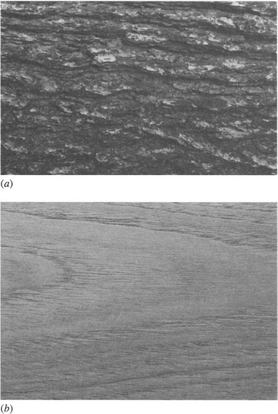
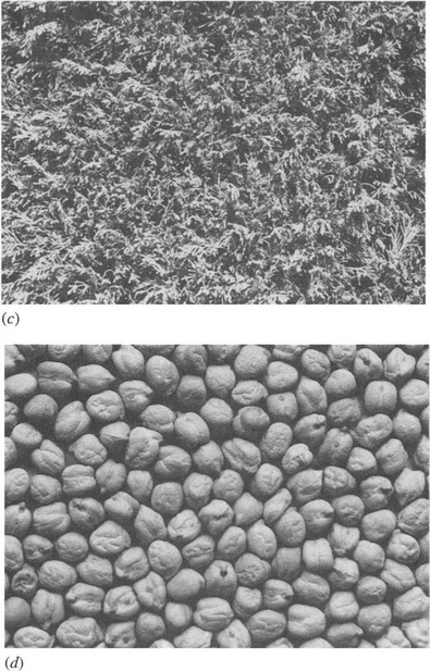
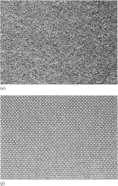
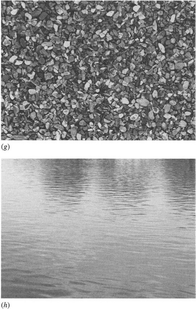
Figure 26.1 A variety of textures. These textures demonstrate the wide variety of familiar textures that are easily recognized from their characteristic intensity patterns.

This definition of texture implies that texture is nonexistent in a surface of uniform intensity, and it does not say anything about how the intensity might be expected to vary or how we might recognize and describe it. Intensity might vary in numerous ways, but if the variation does not have sufficient uniformity, the texture may not be characterized sufficiently closely to permit recognition or segmentation.

We next consider ways in which intensity might vary. It can vary rapidly or slowly, markedly or with low contrast, with a high or low degree of directionality, and with greater or lesser degrees of regularity. This last characteristic is often taken as key: either the textural pattern is regular as for a piece of cloth, or it is random as for a sandy beach or a pile of grass cuttings. However, this ignores the fact that a regular textural pattern is often not wholly regular (again, as for a piece of cloth), or not wholly random (as for a mound of potatoes of similar size). Thus, the degrees of randomness and of regularity will have to be measured and compared when characterizing a texture.

There are more profound things to say about the textures. Often they are derived from tiny objects or components that are themselves similar, but that are placed together in ways ranging from purely random to purely regular—be they bricks in a wall, grains of sand, blades of grass, strands of material, stripes on a shirt, wickerwork on a basket, or a host of other items. In texture analysis it is useful to have a name for the similar textural elements that are replicated over a region of the image: such textural elements are called texels. These considerations lead us to characterize textures in the following ways:

It is quite clear from this discussion that a texture is a complicated entity to measure. The reason is primarily that many parameters are likely to be required to characterize it. In addition, when so many parameters are involved, it is difficult to disentangle the available data and measure the individual values or decide the ones that are most relevant for recognition. And, of course, the statistical nature of many of the parameters is by no means helpful. However, we have so far only attempted to show how complex the situation can be. In the following paragraphs, we attempt to show that quite simple measures can be used to recognize and segment textures in practical situations.

Before proceeding, it is useful to recall that in the analysis of shape a dichotomy exists between available analysis methods. We could, for example, use a set of measures such as circularity, aspect ratio, and so on which would permit a description of the shape, but which would not allow it to be reconstructed. Or we could use descriptors such as skeletons with distance function values, or moments, which would permit full and accurate reconstruction—though the set of descriptors might have been curtailed so that only limited but predictable accuracy was available. In principle, such a reconstruction criterion should be possible with texture. However, in practice there are two levels of reconstruction. In the first, we could reproduce a pattern that, to human eyes, would be indistinguishable from the off-camera texture until one compared the two on a pixel-by-pixel basis. In the second, we could reproduce a textured pattern exactly. The point is that normally textures are partially statistical in nature, so it will be difficult to obtain a pixel-by-pixel match in intensities. Neither, in general, will it be worth aiming to do so. Thus, texture analysis generally only aims at obtaining accurate statistical descriptions of textures, from which apparently identical textures can be reproduced if desired.

At this point it ought to be stated that many workers have contributed to, and used, a wide range of approaches for texture analysis over a period of well over 40 years. The sheer weight of the available material and the statistical nature of it can be daunting for many. It is therefore recommended that those interested in obtaining a quick working view of the subject start by reading Sections 26.2 and 26.4, looking over Sections 26.5 and 26.6, and then proceeding to the end of the chapter. In this way they will bypass much of the literature review material that is part and parcel of a full study of the subject. (Section 26.4 is particularly relevant to practitioners, as it describes the Laws’ texture energy approach which is intuitive, straightforward to apply in both software and hardware, and highly effective in many application areas.)

26.2 Some Basic Approaches to Texture Analysis

In Section 26.1 we defined texture as the characteristic variation in intensity of a region of an image that should allow us to recognize and describe it and to outline its boundaries. In view of the likely statistical nature of textures, this prompts us to characterize texture by the variance in intensity values taken over the whole region of the texture.² However, such an approach will not give a rich enough description of the texture for most purposes and will certainly not provide any possibility of reconstruction. It will also be especially unsuitable in cases where the texels are well defined, or where there is a high degree of periodicity in the texture. On the other hand, for highly periodic textures such as arise with many textiles, it is natural to consider the use of Fourier analysis. In the early days of image analysis, this approach was tested thoroughly, though the results were not always encouraging.

Bajcsy (1973) used a variety of ring and oriented strip filters in the Fourier domain to isolate texture features—an approach that was found to work successfully on natural textures such as grass, sand, and trees. However, there is a general difficulty in using the Fourier power spectrum in that the information is more scattered than might at first be expected. In addition, strong edges and image boundary effects can prevent accurate texture analysis by this method, though Shaming (1974) and Dyer and Rosenfeld (1976) tackled the relevant image aperture problems. Perhaps more important is the fact that the Fourier approach is a global one that is difficult to apply successfully to an image that is to be segmented by texture analysis (Weszka et al., 1976).

Autocorrelation is another obvious approach to texture analysis, since it should show up both local intensity variations and the repeatability of the texture (see Fig. 26.2). In an early study, Kaizer (1955) examined how many pixels an image has to be shifted before the autocorrelation function drops to 1/e of its initial value, and produced a subjective measure of coarseness on this basis. However, Rosenfeld and Troy (1970a, b) later showed that autocorrelation is not a satisfactory measure of coarseness. In addition, autocorrelation is not a very good discriminator of isotropy in natural textures. Hence, workers were quick to take up the co-occurrence matrix approach introduced by Haralick et al. in 1973. This approach not only replaced the use of autocorrelation but during the 1970s became to a large degree the standard approach to texture analysis.

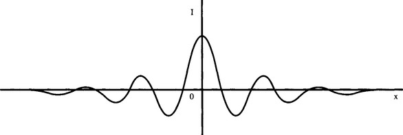
Figure 26.2 Use of autocorrelation function for texture analysis. This diagram shows the possible 1-D profile of the autocorrelation function for a piece of material in which the weave is subject to significant spatial variation. Notice that the periodicity of the autocorrelation function is damped down over quite a short distance.

26.3 Gray-level Co-occurrence Matrices

The gray-level co-occurrence matrix approach³ is based on studies of the statistics of pixel intensity distributions. As hinted above with regard to the variance in pixel intensity values, single-pixel statistics do not provide rich enough descriptions of textures for practical applications. Thus, it is natural to consider second-order statistics obtained by considering pairs of pixels in certain spatial relations to each other. Hence, co-occurrence matrices are used, which express the relative frequencies (or probabilities) P(i, j|d, θ) with which two pixels having relative polar coordinates (d, θ) appear with intensities i, j. The co-occurrence matrices provide raw numerical data on the texture, though these data must be condensed to relatively few numbers before it can be used to classify the texture. The early paper by Haralick et al. (1973) presented 14 such measures, and these were used successfully for classification of many types of materials (including, for example, wood, corn, grass, and water). However, Conners and Harlow (1980a) found that only five of these measures were normally used, viz. “energy,” “entropy,” “correlation,” “local homogeneity,” and “inertia.” (Note that these names do not provide much indication of the modes of operation of the respective operators.)

To obtain a more detailed idea of the operation of the technique, consider the co-occurrence matrix shown in Fig. 26.3. This corresponds to a nearly uniform image containing a single region in which the pixel intensities are subject to an approximately Gaussian noise distribution, the attention being on pairs of pixels at a constant vector distance d = (d, θ) from each other. Next consider the co-occurrence matrix shown in Fig. 26.4, which corresponds to an almost noiseless image with several nearly uniform image regions. In this case, the two pixels in each pair may correspond either to the same image regions or to different ones, though if d is small they will only correspond to adjacent image regions. Thus, we have a set of N on-diagonal patches in the co-occurrence matrix, but only a limited number L of the possible number M of off-diagonal patches linking them, where and L ≤ M. (Typically, L will be of order N rather than N².) With textured images, if the texture is not too strong, it may by modeled as noise, and the N + L patches in the image will be larger but still not overlapping. However, in more complex cases the possibility of segmentation using the co-occurrence matrices will depend on the extent to which d can be chosen to prevent the patches from overlapping. Since many textures are directional, careful choice of θ will help with this task, though the optimum value of d will depend on several other characteristics of the texture.

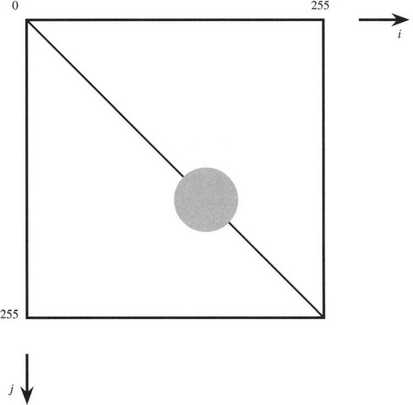
Figure 26.3 Co-occurrence matrix for a nearly uniform gray-scale image with superimposed Gaussian noise. Here the intensity variation is taken to be almost continuous. Normal convention is followed by making the j index increase downwards, as for a table of discrete values (cf. Fig. 26.4).

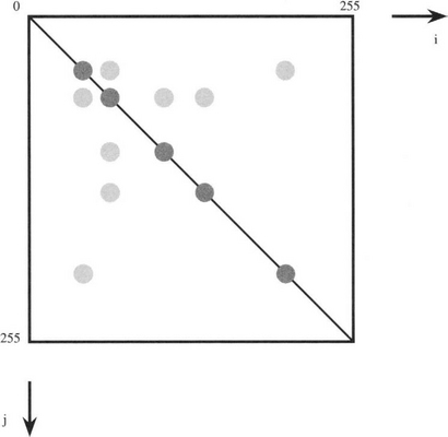
Figure 26.4 Co-occurrence matrix for an image with several distinct regions of nearly constant intensity. Again, the leading diagonal of the diagram is from top left to bottom right (cf. Figs. 26.2 and 26.4).

As a further illustration, we consider the small image shown in Fig. 26.5a. To produce the co-occurrence matrices for a given value of d, we merely need to calculate the number of cases for which pixels a distance d apart have intensity values i and j. Here, we content ourselves with the two cases d = (1, 0) and d = (1, π/2). We thus obtain the matrices shown in Fig. 26.5b and c.

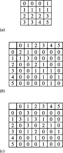
Figure 26.5 Co-occurrence matrices for a small image. (a) shows the original image; (b) shows the resulting co-occurrence matrix for d = (1, 0), and (c) shows the matrix for d = (1, π/2). Note that even in this simple case the matrices contain more data than the original image.

This simple example demonstrates that the amount of data in the matrices is liable to be many times more than in the original image—a situation that is exacerbated in more complex cases by the number of values of d and θ that is required to accurately represent the texture. In addition, the number of gray levels will normally be closer to 256 than to 6, and the amount of matrix data varies as the square of this number. Finally, we should notice that the co-occurrence matrices merely provide a new representation: they do not themselves solve the recognition problem.

These factors mean that the gray-scale has to be compressed into a much smaller set of values, and careful choice of specific sample d, θ values must be made. In most cases, it is not obvious how such a choice should be made, and it is even more difficult to arrange for it to be made automatically. In addition, various functions of the matrix data must be tested before the texture can be properly characterized and classified.

These problems with the co-occurrence matrix approach have been tackled in many ways: just two are mentioned here. The first is to ignore the distinction between opposite directions in the image, thereby reducing storage by 50%. The second is to work with differences between gray levels. This amounts to performing a summation in the co-occurrence matrices along axes parallel to the main diagonal of the matrix. The result is a set of first-order difference statistics. Although these modifications have given some additional impetus to the approach, the 1980s saw a highly significant diversification of methods for the analysis of textures. Of these, Laws’ approach (1979, 1980a, b) is important in that it has led to other developments that provide a systematic, adaptive means of conducting texture analysis. This approach is covered in the following section.

26.4 Laws’ Texture Energy Approach

In 1979 and 1980, Laws presented his novel texture energy approach to texture analysis (1979, 1980a, b). This involved the application of simple filters to digital images. The basic filters he used were common Gaussian, edge detector, and Laplacian-type filters, and were designed to highlight points of high “texture energy” in the image. By identifying these high-energy points, smoothing the various filtered images, and pooling the information from them he was able to characterize textures highly efficiently and in a manner compatible with pipelined hardware implementations. As remarked earlier, Laws’ approach has strongly influenced much subsequent work, and it is therefore worth considering it here in some detail.

The Laws’ masks are constructed by convolving together just three basic 1 × 3 masks:

     (26.1)

     (26.2)

     (26.3)

The initial letters of these masks indicate Local averaging, Edge detection, and Spot detection. These basic masks span the entire 1 × 3 subspace and form a complete set. Similarly, the 1 × 5 masks obtained by convolving pairs of these 1 × 3 masks together form a complete set:⁴

     (26.4)

     (26.5)

     (26.6)

     (26.7)

     (26.8)

(Here the initial letters are as before, with the addition of Ripple detection and Wave detection.) We can also use matrix multiplication (see also Section 3.6) to combine the 1 × 3 and a similar set of 3 × 1 masks to obtain nine 3 × 3 masks—for example:

     (26.9)

The resulting set of masks also forms a complete set (Fig. 26.6). Note that two of these masks are identical to the Sobel operator masks. The corresponding 5 × 5 masks are entirely similar but are not considered in detail here as all relevant principles are illustrated by the 3 × 3 masks.

Figure 26.6 The nine 3 × 3 Laws masks.

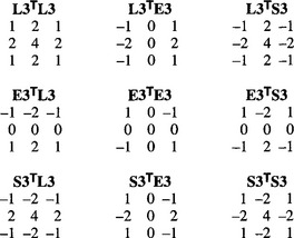
All such sets of masks include one whose components do not average to zero. Thus, it is less useful for texture analysis since it will give results dependent more on image intensity than on texture. The remainder are sensitive to edge points, spots, lines, and combinations of these.

Having produced images that indicate local edginess and so on, the next stage is to deduce the local magnitudes of these quantities. These magnitudes are then smoothed over a fair-sized region rather greater than the basic filter mask size (e.g., Laws used a 15 × 15 smoothing window after applying his 3 × 3 masks). The effect is to smooth over the gaps between the texture edges and other microfeatures. At this point, the image has been transformed into a vector image, each component of which represents energy of a different type. Although Laws (1980b) used both squared magnitudes and absolute magnitudes to estimate texture energy, the squared magnitude corresponded to true energy and gave a better response, whereas absolute magnitudes require less computation:

     (26.10)

F(i, j) being the local magnitude of a typical microfeature that is smoothed at a general scan position (l, m) in a (2p + 1) × (2p + 1) window.

A further stage is required to combine the various energies in a number of different ways, providing several outputs that can be fed into a classifier to decide upon the particular type of texture at each pixel location (Fig. 26.7). If necessary, principal components analysis is used at this point to help select a suitable set of intermediate outputs.

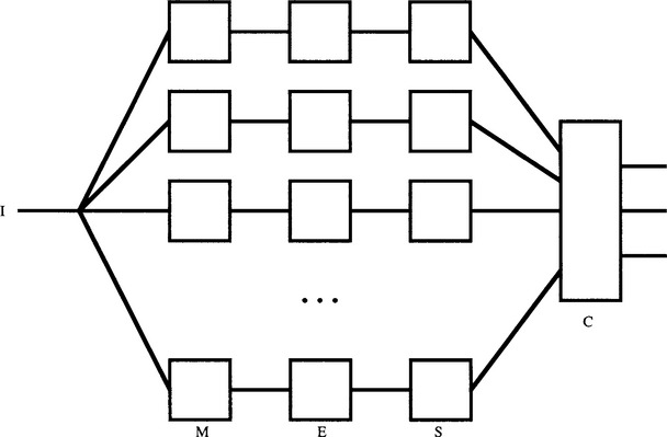
Figure 26.7 Basic form for a Laws texture classifier. Here I is the incoming image, M represents the microfeature calculation, E the energy calculation, S the smoothing, and C the final classification.

Laws’ method resulted in excellent classification accuracy quoted at (for example) 87% compared with 72% for the co-occurrence matrix method, when applied to a composite texture image of grass, raffia, sand, wool, pigskin, leather, water, and wood (Laws, 1980b). Laws also found that the histogram equalization normally applied to images to eliminate first-order differences in texture field gray-scale distributions produced little improvement in this case.

Pietikäinen et al. (1983) conducted research to determine whether the precise coefficients used in Laws’ masks are responsible for the performance of his method. They found that as long as the general forms of the masks were retained, performance did not deteriorate and could in some instances be improved. They were able to confirm that Laws’ texture energy measures are more powerful than measures based on pairs of pixels (i.e., co-occurrence matrices), although Unser (1986) later questioned the generality of this result.

26.5 Ade’s Eigenfilter Approach

In 1983, Ade investigated the theory underlying Laws’ approach and developed a revised rationale in terms of eigenfilters. He took all possible pairs of pixels within a3 × 3 window and characterized the image intensity data by a 9 × 9 covariance matrix. He then determined the eigenvectors required to diagonalize this matrix. These correspond to filter masks similar to Laws’ masks (i.e., use of these “eigenfilter” masks produces images that are principal component images for the given texture). Furthermore, each eigenvalue gives that part of the variance of the original image that can be extracted by the corresponding filter. Essentially, the variances give an exhaustive description of a given texture in terms of the texture of the images from which the covariance matrix was originally derived. The filters that give rise to low variances can be taken to be relatively unimportant for texture recognition.

It will be useful to illustrate the technique for a 3 × 3 window. Here we follow Ade (1983) in numbering the pixels within a 3 × 3 window in scan order:

This leads to a 9 × 9 covariance matrix for describing relationships between pixel intensities within a 3 × 3 window, as stated above. At this point, we recall that we are describing a texture, and assuming that its properties are not synchronous with the pixel tessellation, we would expect various coefficients of the covariance matrix C to be equal. For example, C₂₄ should equal C₅₇; in addition, C₅₇ must equal C₇₅.

It is worth pursuing this matter, as a reduced number of parameters will lead to increased accuracy in determining the remaining ones. There are[inlinefigure] ways of selecting pairs of pixels, but there are only 12 distinct spatial relationships between pixels if we disregard translations of whole pairs—or 13 if we include the null vector in the set (see Table 26.1). Thus, the covariance matrix (see Section 24.10) takes the form:

     (26.11)

Cis symmetrical; the eigenvalues of a real symmetrical covariance matrix are real and positive; and the eigenvectors are mutually orthogonal (see Section 24.10). In addition, the eigenfilters thus produced reflect the proper structure of the texture being studied and are ideally suited to characterizing it. For example, for a texture with a prominent highly directional pattern, there will be one or more high-energy eigenvalues, with eigenfilters having strong directionality in the corresponding direction.

26.6 Appraisal of the Laws and Ade Approaches

At this point, it will be worthwhile to compare the Laws and Ade approaches more carefully. In the Laws approach, standard filters are used, texture energy images are produced, and then principal components analysis may be applied to lead to recognition, whereas in the Ade approach, special filters (the eigenfilters) are applied, incorporating the results of principal components analysis, following which texture energy measures are calculated and a suitable number of these are applied for recognition.

The Ade approach is superior to the extent that it permits low-value energy components to be eliminated early on, thereby saving computation. For example, in Ade’s application, the first five of the nine components contain 99.1% of the total texture energy, so the remainder can definitely be ignored. In addition, it would appear that another two of the components containing, respectively, 1.9% and 0.7% of the energy could also be ignored, with little loss of recognition accuracy. In some applications, however, textures could vary continually, and it may well not be advantageous to fine-tune a method to the particular data pertaining at any one time.⁵ In addition, to do so may prevent an implementation from having wide generality or (in the case of hardware implementations) being so cost-effective. There is therefore still a case for employing the simplest possible complete set of masks and using the Laws approach. However, Unser and Ade (1984) have adopted the Ade approach and report encouraging results. More recently, the work of Dewaele et al. (1988) has built solidly on the Ade eigenfilter approach.

In 1986, Unser developed a more general version of the Ade technique, which also covered the methods of Faugeras (1978), Granlund (1980), and Wermser and Liedtke (1982). In this approach not only is performance optimized for texture classification but also it is optimized for discrimination between two textures by simultaneous diagonalization of two covariance matrices. The method has been developed further by Unser and Eden (1989, 1990). This work makes a careful analysis of the use of nonlinear detectors. As a result, two levels of nonlinearity are employed, one immediately after the linear filters and designed (by employing a specific Gaussian texture model) to feed the smoothing stage with genuine variance or other suitable measures, and the other after the spatial smoothing stage to counteract the effect of the earlier filter, and aiming to provide a feature value that is in the same units as the input signal. In practical terms this means having the capability for providing an r.m.s. texture signal from each of the linear filter channels.

Overall, the originally intuitive Laws approach emerged during the 1980s as a serious alternative to the co-occurrence matrix approach. It is as well to note that alternative methods that are potentially superior have also been devised. See, for example, the local rank correlation method of Harwood et al. (1985), and the forced-choice method of Vistnes (1989) for finding edges between different textures, which apparently has considerably better accuracy than the Laws approach. Vistnes’ (1989) investigation concludes that the Laws approach is limited by (1) the small scale of the masks which can miss larger-scale textural structures, and (2) the fact that the texture energy smoothing operation blurs the texture feature values across the edge. The second finding (or the even worse situation where a third class of texture appears to be located in the region of the border between two textures) has also been noted by Hsiao and Sawchuk (1989, 1990) who applied an improved technique for feature smoothing. They also used probabilistic relaxation for enforcing spatial organization on the resulting data.

26.7 Fractal-based Measures of Texture

Fractals, an important new approach to texture analysis that arose in the 1980s, incorporate the observation due to Mandelbrot (1982) that measurements of the length of a coastline (for example) will vary with the size of the measuring tool used for the purpose, since details smaller than the size of the tool will be missed. If the size of the measuring tool is taken as λ, the measured quantity will be M = nλ^D, where D is known as the fractal dimension and must in general be larger than the immediate geometric dimension if correct measurements are to result. (For a coastline we will thus have D > 2.) Thus, when measurements are being made of 2-D textures, it is found that D can take values from 2.0 to at least 2.8 (Pentland, 1984). Interestingly, these values of D have been found to correspond roughly to subjective measures of the roughness of the surface being inspected (Pentland, 1984). The concept of fractal dimension is a mathematical one, which can only apply over a range of scales for physical surfaces. Nevertheless, if the concept is not applied over such a range of scales (as is the case for most existing texture analysis methods), then the measures of texture that result cannot be scale invariant. The texture measure will therefore have to be recalibrated for every possible scale at which it is applied. This would be highly inconvenient, so fractal concepts strike at the heart of the texture measurement problem. (Seemingly, ignoring them would only be valid if, for example, textiles or cornfields were being inspected from a fixed height.) At the same time, it is fortunate that fractal dimension appears to represent a quantity as useful as surface roughness. Furthermore, the fact that it reduces the number of textural attributes from the initially large numbers associated with certain other methods of textural measurement (such as co-occurrence matrices) is also something of an advantage.

Since Pentland (1984) put forward these arguments, other workers have had problems with the approach. For example, reducing all textural measurements to the single measure D cannot permit all textures to be distinguished (Keller et al., 1989). Hence, an attempt has been made to define further fractal-based measures. Mandelbrot himself contributed the concept of lacunarity and in 1982 provided one definition, whereas Voss (1986) and Keller et al. (1989) provided further definitions. These definitions differ in mathematical detail, but all three appear to measure a sort of texture mark–space ratio that is distinct from average surface roughness. Lacunarity seems to give good separation for most materials having similar fractal dimensions, though Keller et al. proposed further research to combine these measures with other statistical and structural measurements. Ultimately, an important problem of texture analysis will be to determine how many features are required to distinguish different materials and surfaces reliably, while not making the number so large that computation becomes excessive, or (perhaps more important) so that the raw data are unable to support so many features (i.e., so that the features that are chosen are not all statistically significant—see Section 24.5). Meanwhile, it should be noted that the fractal measures currently being used require considerable computation that may not be justified for applications such as automated inspection.

Finally, note that Gårding (1988) found that fractal dimension is not always equivalent to subjective judgments of roughness. In particular, he revealed that a region of Gaussian noise of low amplitude superimposed on a constant gray level will have a fractal dimension that approaches 3.0. This is a rather high value, which is contrary to our judgment of such surfaces as being quite smooth. (An interpretation of this result is that highly noisy textures appear exactly like 3-D landscapes in relief!)

26.8 Shape from Texture

This topic in texture analysis also developed strongly during the 1980s. After early work by Bajcsy and Liebermann (1976) for the case of planar surfaces, Witkin (1981) and Kender (1983) significantly extended this work and at the same time laid the foundations for general development of the whole subject. Many papers have followed (e.g., Aloimonos and Swain, 1985; Aloimonos, 1988; Katatani and Chou, 1989; Blostein and Ahuja, 1989; Stone, 1990); there is no space to cover all this work here. In general, workers have studied how an assumed standard texel shape is distorted and its size changed by 3-D projections; they then relate this to the local orientation of the surface. Since the texel distortion varies as the cosine of the angle between the line of sight and the local normal to the surface plane, essentially similar “reflectance map” analysis is required as in the case of shape-from-shading estimation. An alternative approach adopted by Chang et al. (1987) involves texture discrimination by projective invariants (see Chapter 19). More recently, Singh and Ramakrishna (1990) exploited shadows and integrated the information available from texture and from shadows. The problem is that in many situations insufficient data arise from either source taken on its own. Although the results of Singh and Ramakrishna are only preliminary, they indicate the direction that texture work must develop if it is to be used in practical image understanding systems.

26.9 Markov Random Field Models of Texture

Markov models have long been used for texture synthesis to help with the generation of realistic images. They have also proved increasingly useful for texture analysis. In essence, a Markov model is a one-dimensional construct in which the intensity at any pixel depends only upon the intensity of the previous pixel in a chain and upon a transition probability matrix. For images, this is too weak a characterization, and various more complex constructs have been devised. Interest in such models dates from as early as 1965 (Abend et al., 1965) (see also Woods, 1972), though such work is accorded no great significance in Haralick’s extensive review of 1979. However, by 1982 the situation was starting to change (Hansen and Elliott, 1982), and a considerable amount of further work was soon being published (e.g., Cross and Jain, 1983; Geman and Geman, 1984; Derin and Elliott, 1987) as Gibbs distributions came to be used for characterizing Markov random fields. In fact, Ising’s much earlier work in statistical mechanics (1925) was the starting point for these developments.

Available space does not permit details of these algorithms to be given here. By 1987 impressive results for texture segmentation of real scenes were being achieved using this approach (Derin and Elliott, 1987; Cohen and Cooper, 1987). In particular, the approach appears to be able to cope with highly irregular boundaries, local boundary estimation errors normally lying between 0 and 3 pixels. Unfortunately, these algorithms depend on iterative processing of the image and so tend to require considerable amounts of computation. Cohen and Cooper (1987) state that little processing is required, though there is an inbuilt assumption that a suitable highly parallel processor will be available. On the other hand, they also showed that a hierarchical segmentation algorithm can achieve considerable computational savings, which are greatest when the texture fields have spatially constant parameters.

Finally, stochastic models are useful not only for modeling texture and segmenting one textured region from another, but also for more general segmentation purposes, including cases where boundary edges are quite noisy (Geman, 1987). The fact that a method such as this effectively takes texture as a mere special case demonstrates the power of the whole approach.

26.10 Structural Approaches to Texture Analysis

It has already been remarked that textures approximate to a basic textural element or primitive that is replicated in a more or less regular manner. Structural approaches to texture analysis aim to discern the textural primitive and to determine the underlying gross structure of the texture. Early work (e.g. Pickett, 1970) suggested the structural approach, though little research on these lines was carried out until the late 1970s. Work of this type has been described by Davis (1979), Conners and Harlow (1980b), Matsuyama et al. (1982), Vilnrotter et al. (1986), and Kim and Park (1990). An unusual and interesting paper by Kass and Witkin (1987) shows how oriented patterns from wood grain, straw, fabric, and fingerprints, as well as spectrograms and seismic patterns, can be analyzed. The method adopted involves building up a flow coordinate system for the image, though the method rests more on edge pattern orientation analysis than on more usual texture analysis procedures. A similar statement may be made about the topologically invariant texture descriptor method of Eichmann and Kasparis (1988), which relies on Hough transforms for finding line structures in highly structured textiles. More recently, pyramidal approaches have been applied to structural texture segmentation (Lam and Ip, 1994).

26.11 Concluding Remarks

In this chapter we have seen the difficulties of analyzing textures. These difficulties arise from the potential of textures, and in many cases the frighteningly real complexities of textures—not least from the fact that their properties are often largely statistical in nature. The erstwhile widely used gray-scale co-occurrence matrix approach has been seen to have distinct computational shortcomings. First, many co-occurrence matrices are in principle required (with different values of d and θ) in order to adequately describe a given texture; second, the co-occurrence matrices can be very large and, paradoxically, may hold more data than the image data they are characterizing—especially if the range of gray-scale values is large. In addition, many sets of co-occurrence matrices may be needed to allow for variation of the texture over the image, and if necessary to initiate segmentation. Hence co-occurrence matrices need to be significantly compressed, though in most cases it is not at all obvious a priori how this should be achieved. It is even more difficult to arrange for it to be carried out automatically. This probably explains why attention shifted during the 1980s to other approaches, including particularly Laws’ technique and its variations (especially that of Ade). Other natural developments were fractal-based measures and the attention given to Markov approaches. A further important development, which could not be discussed here for space reasons, is the Gabor filter technique (see, for example, Jain and Farrokhnia, 1991).

During the past 15 years or so, considerable attention has also been paid to neural network methodologies, because these are able to extract the rules underlying the construction of textures, apparently without the need for analytic or statistical effort. Although neural networks have been able to achieve certain practical goals in actual applications, there is little firm evidence whether they are actually superior to Markov or other methods because conclusive comparative investigations have still not been performed. However, they do seem to offer solutions requiring minimal computational load.

26.12 Bibliographical and Historical Notes

Early work on texture analysis was carried out by Haralick et al. (1973), and in 1976 Weska and Rosenfeld applied textural analysis to materials inspection. The area was reviewed by Zucker (1976a) and by Haralick (1979), and excellent accounts appear in the books by Ballard and Brown (1982) and Levine (1985).

At the end of the 1970s, the Laws technique (1979, 1980a, b) emerged on the scene (which until then had been dominated by the co-occurrence matrix approach), and led to the principal components approach of Ade (1983), which was further developed by Dewaele et al. (1988), Unser and Eden (1989, 1990), and others. For related work on the optimization of convolution filters, see Benke and Skinner (1987). The direction taken by Laws was particularly valuable as it showed how texture analysis could be implemented straightforwardly and in a manner consistent with real-time applications such as inspection.

The 1980s also saw other new developments, such as the fractal approach led by Pentland (1984), and a great amount of work on Markov random field models of texture. Here the work of Hansen and Elliott (1982) was very formative, though the names Cross, Derin, D. Geman, S. Geman, and Jain come up repeatedly in this context (see Section 26.9). Bajcsy and Liebermann (1976), Witkin (1981), and Kender (1983) pioneered the shape from texture concept, which has received much attention ever since. Finally, the last 10 to 15 years have seen much work on the application of neural networks to texture analysis, for example, Greenhill and Davies (1993) and Patel et al. (1994).

A number of reviews and useful comparative studies have been made, including Van Gool et al. (1985), Du Buf et al. (1990), Ohanian and Dubes (1992), and Reed and Du Buf (1993). For further work on texture analysis related to inspection for faults and foreign objects, see Chapter 22.

Recent developments include further work with automated visual inspection in mind (Davies, 2000c; Tsai and Huang, 2003; Ojala et al., 2002; Manthalkar et al., 2003; Pun and Lee, 2003), although several of these papers also cite medical, remote sensing, and other applications, as the authors are aware of the generic nature of their work. Of these papers, the last three are specifically aimed at rotation invariant texture classification, and the last one, Pun and Lee, also aims at scale invariance. In previous years there has not been quite this emphasis on rotation invariance, though it is by no means a new topic. Other work (Clerc and Mallat, 2002) is concerned with recovering shape from texture via a texture gradient equation, while Ma et al. (2003) are particularly concerned with person identification based on iris textures. Mirmehdi and Petrou (2000) describe an in-depth investigation of color texture segmentation. In this context, the importance of “wavelets” ⁶ as an increasingly used technique of texture analysis with interesting applications (such as human iris recognition) should be noted (e.g., Daugman, 1993, 2003).

Finally, in a particularly exciting advance, Spence et al. (2003) have managed to eliminate texture by using photometric stereo to find the underlying surface shape (or “bump map”), following which they have been able to perform impressive reconstructions, including texture, from a variety of viewpoints. McGunnigle and Chantler (2003) have shown that this kind of technique can also reveal hidden writing on textured surfaces, where only pen pressure marks have been made. Similarly, Pan et al. (2004) have shown how texture can be eliminated from ancient tablets (in particular those made of lead and wood) to reveal clear images of the writing underneath.