
CHAPTER 20 Egomotion and Related Tasks
20.1 Introduction
Mechatronics is the study of mechanisms and the electronic systems that are needed to provide them with intelligent control. It has applications in a wide variety of areas, including industry, commerce, transport, space, and even the health service. For instance, robots can be used in principle–and often in practice–for mowing lawns, clearing rubbish, driving vehicles, effecting bomb disposal, carrying out reconnaissance, performing delicate operations, and executing automatic assembly tasks. A related task is that of automated inspection for quality control, though in that case the robots take the form of trapdoors or air jets that divert defective items into reject bins (Chapter 22). There are several categories of mechanisms and robots: mobile robots, which include robot vacuum cleaners and other autonomous vehicles; stationary robots with arms that can spray cars on production lines or assemble television sets; and robots that do not have discernible arms but that insert components into printed circuit boards or inspect food products or brake hubs and reject faulty items.
By definition, all mechatronic systems control the processes they are part of, and to achieve this control they need sensors of various sorts. Sensors can be tactile, ultrasonic, or visual or can involve one of a number of other modalities, some of which provide images that can be handled in the same way as normal visual images. Instances include ultrasonic, infrared, thermographic, X-ray, and ultraviolet images. In this chapter we are concerned primarily with these sorts of visual image, though some mechatronic applications do not involve this general class of input. However, far too many mechatronic applications use visual images for control than we can deal with here. Thus, we shall concentrate on autonomous mobile robots and related egomotion1 problems.
20.2 Autonomous Mobile Robots
Mobile robots are poised to invade the human living space at an ever increasing rate. The mechanical technology is already in place, and the sensing systems required to guide them have been evolving for many years and are sufficiently mature for serious, though perhaps not ambitious, application. For example, robot lawnmowers, robot vacuum cleaners, robot window cleaners, robot rubbish gatherers, and robot weed-sprayers have been produced, but more ambitious, autonomous vehicles are held back largely because of the risks involved when humans inhabit the same areas–and in case of accidents, litigation could pose serious problems. Indeed, attempting to advance too quickly could set the industry back.
In addition to safety considerations, there are other practical issues such as speed of operation and implementation cost. The problems of applying mobile robots have not all been solved, especially in light of these practical issues. Ignoring the end use of the robot, one of the main things still to be engineered is how the robot is to guide itself safely in territory that will be populated by humans and by other robots. Autonomous guidance involves sensing, scene interpretation, and navigation. On a limited scale, a floor polishing robot could proceed until it bumps into an object and then take evading action. In this case tactile sensing is required. However, ultrasonic devices permit proximity sensing and appreciation that other objects that have to be avoided are nearby. Here the need for planning is beginning to be felt (Kanesalingam et al., 1998). However, serious planning and navigation are probably possible only when vision sensing is used, as vision sensing is remotely instituted and is rich in information content and flow rate.
Although vision sensing provides an extremely rich flow of information that potentially is exceptionally valuable for autonomous control and path planning, the interpretation task is considerable. In addition, it has to be remembered that mobile robots will be moving at walking speed indoors, and at much greater speeds outdoors, so a significant real-time processing problem arises. However, it seems that stereo vision offers limited advantage in that (1) the additional information requires additional processing and (2) it does not offer substantial advantages in 3-D scene interpretation at distances of more than a few meters. On the other hand, stereo can help the vision system to cue into the complex information present in the incoming images. Thus, if stereo is not to be used, reliable cues have to be found in monocular images. A widely used means by which such cues can be obtained is by vanishing point (VP) detection. VPs are all too evident to humans in the sort of environment in which they live and work. In particular, factories, office-blocks, hospitals, universities, and outdoor city scenes all tend to contain many structures that are composed not only of straight lines and planes but also of rectangular blocks and towers (Fig. 20.1).
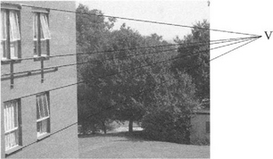
Figure 20.1 Vanishing point formation. In this case, parallel lines in space appear to converge to a vanishing point to the right of the image. Although the vanishing point V is only marginally outside the image, in many other cases it lies a considerable distance away.
Vanishing points are useful in several ways. They confirm that various lines in the scene arise from parallel lines in the environment; they help to identify where the ground plane is; they permit local scale to be deduced (e.g., objects on the ground plane have width that is referable to, and a known fraction of, the local width of the ground plane); and they permit an estimate to be made of distance along the ground plane, by measuring the distance from the relevant image point to the VP. Thus, they are useful for initiating the process of recognizing and measuring objects, determining their positions and orientations, and helping with the task of navigation. Section 20.4 covers location of VPs, and Section 20.6 examines the process of navigation and path planning in greater detail.
20.3 Active Vision
The term active vision has several meanings, and it is important to differentiate carefully between them. First, there is a connotation that comes from radar, active radar being different from passive radar in that the aircraft being sensed deliberately returns a special signal that is able to identify it. This is not a normal connotation in vision. Instead, active vision is taken to mean one of two things: (1) moving the camera around to focus on and attend to a particular item of current interest in the environment; or (2) attending to a particular item or region in the image and interacting dynamically with it until an acceptable interpretation is arrived at. In either case, there is a focus of attention, and the vision system spends its time actively pursuing and analyzing what is present in the scene, rather than blandly interpreting the scene as a whole and attempting to recognize everything. In active vision, it is up to a higher level processor to identify items of interest and to ask, and answer, strategic questions about them.
Although these two modes of active vision may seem very similar, they have evolved to be quite distinct. In the first mode, the activity takes place largely in terms of what the camera may be made to look at. In the second, the activity takes place at the processing level, and active agents such as snakes are used to analyze different parts of the received image. Thus, a snake may initially be looped loosely around the whole region of an object and will then gradually move inward until it has sensed exactly where the object is. This is achieved by interacting intelligently with the object region and interrogating it until a viable solution is reached. In one sense, both schemes are carrying out interrogation, and in that sense active vision is being undertaken in each case. However, each scheme carries a different emphasis. What is important in the case of the moving camera is that recording and memorizing the whole of a scene in all directions around a robot station is necessarily a costly process, and one for which a complete interpretation is unlikely to be fully utilized. It is wasteful to gather information that will not be used later. It is better to concentrate on finding the part of the scene that is currently most useful and to narrow its scope and enhance its quality so that really useful answers can be found (see, for example, Yazdi and King, 1998). This approach mimics the human interrogation of scenes, which involves making “saccades” from one focus of attention to another, thus obtaining a progressive understanding of what is happening in the environment.
The active vision approach is useful for practical control of real robot limbs, but it is even more vital for mobile robots that have to guide themselves around the factory, hospital, office-block, or (in the case of robot vehicles) along the highway. In such cases it is relevant to update only those parts of the scene that give the information needed for the main task–that of safe guidance and navigation.
20.4 Vanishing Point Detection
We next consider how VPs can be detected. Generally, the process is undertaken in two stages: (1) locate all the straight lines in the image; (2) find those lines that pass through common points and deduce which must be VPs. Stage 1 is in principle a straightforward application of the Hough transform, though how straightforward depends on whether some of the lines are texture edges, which are difficult to locate accurately and consistently. Stage 2 is, in effect, another Hough transform in which peaks are located in a parameter space congruent to the image space, in which all points on lines are accumulated. Points on extended lines as well as those on the lines themselves have to be accumulated. Unfortunately, complications arise as VPs may be outside the confines of the initial image space (Fig. 20.1). Extending the image space can help, but there is no guarantee that this will work. In addition, accuracy of location may be poor when the lines leading to a VP converge at a small angle. Finally, the density of votes accumulated in the VP parameter space may (even with the application of suitable point spread functions) be so low that sensitivity of detection will be negligible. Thus, special techniques are necessary to guarantee success.
Perhaps the most important technique for detecting VPs is to use the surface of a Gaussian sphere as the parameter space (Magee and Aggarwal, 1984). Here, a unit sphere S is constructed around the center of projection of the camera, and S is used as a parameter space, instead of an additional image plane. Thus, VPs appear at convenient positions at finite distances, and infinite distances are ruled out (Fig. 20.2). Notice that there is a one-to-one correspondence between each point on the extended image plane and each point on the front half of the Gaussian sphere (the back half is not used). Nevertheless, using the Gaussian sphere gives rise to problems when analyzing the vote patterns as these are not deposited uniformly over the sphere. In addition, large numbers of irrelevant votes are cast when lines do not pass through actual VPs as they do not originate from lines that are parallel to other lines in the scene. It would be better if all the votes that were cast at isolated peaks corresponded to likely VPs. To help ensure that only useful votes are cast, pairs of lines are taken, and the VPs that would arise if each pair of lines were actually parallel lines in the scene are recorded as votes in the parameter space. If this procedure is implemented for all pairs of lines (or for all pairs of edge segments), all necessary peaks will be recorded in the parameter space, and the amount of unnecessary clutter will be drastically reduced. However, this method for casting votes is not achieved without cost, as the computational load will be proportional to the number of pairs of edge segments, or, alternatively, the number of pairs of lines. If there are N lines, the number of pairs is ![]() , which is proportional to N2 if N is large.
, which is proportional to N2 if N is large.
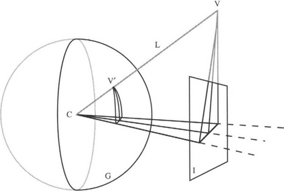
Figure 20.2 Use of Gaussian sphere for vanishing point detection. In this case, the vanishing point V is shown well above the input image I. To be sure of detecting such points, the surface of the Gaussian sphere G is used as the parameter space for accumulating vanishing point votes. Also marked in the figure are the projection line L from the center of projection C to V, and V’, which is the position of the vanishing point on G.
After the Gaussian sphere has been used to locate the peaks corresponding to the VPs, the VPs can, where possible, be recorded in the image space. However, the important step is the initial search to determine which of the initial lines or line segments correspond to the VPs and which correspond to isolated lines or mere clutter. Once the right line assignments have been made, there is considerably greater certainty in the interpretation of the images. By way of confirmation, for a moving robot there should be some correspondence between the VPs seen in successive images.
20.5 Navigation for Autonomous Mobile Robots
When a mobile robot is proceeding down a corridor, the field of view will usually contain at least four lines that converge to a VP situated in the middle of the corridor (Fig. 20.3a). In many cases this VP can be used for navigation purposes. For example, the robot can steer so that the VP is in the very center of the field of view, thus giving maximum clearance with the corridor walls. It can also check that other objects do not come between it and the VP. To simplify the latter process, the floor region in front of the robot should be checked for continuity. Such actions can be taken by examining the image space itself. Indeed, both navigation and obstacle detection can be carried out by scrutinizing the image space, without appeal to special navigation models that map out the entire working area.
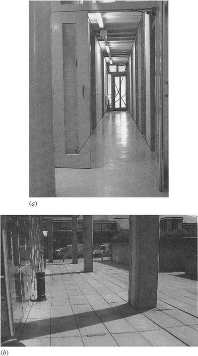
Figure 20.3 Navigational problems posed by obstacles. (a) View of a corridor with four lines converging to a vanishing point, and a narrowed entrance to be negotiated. (b) View of a path with various pillars and bollards to be negotiated. (c) Plan view of (b) showing what can be deduced by examination of the ground plane in (b): only walls W that can be seen from the viewpoint (marked A) are drawn; however, the pillars P, bollards B, and litter-bin L (which are easily recognizable) are in full.
Although this procedure may be sufficient for guiding a vacuum cleaner, more advanced mobile robots will have to make mapping, path planning, and navigational modeling part of a detailed high-level analysis of the situation (Kortenkamp et al., 1998). This will apply if the corridor has several low obstacles such as chairs, wastepaper bins, and display tables, or if a path has obstacles such as bollards or pillars (Fig. 20.3b, c); but will a fortiori be necessary if the robot is running a maze (as in the “Robot Micromouse” contests). In such cases, the robot will have only limited knowledge and visibility of the working area, and the natural representation for thinking about the situation and path planning is a plan view model of the working area. This plan will gradually be augmented as more and more data come to light. The following section indicates how a (partial) plan view can be calculated for each individual frame obtained by the camera. The overall plan construction algorithm is given in Table 20.1.
Table 20.1 Overall algorithm for constructing plan view of ground plane. This table gives the basic steps for constructing a plan view of the ground plane. For simplicity each input image is treated separately until the last few stages, though more sophisticated implementations would adopt a more holistic strategy.
| Steps in Algorithm | |
|---|---|
| • | Perform edge detection. |
| • | Locate straight lines using the Hough transform. |
| • | Find VPs using a further Hough transform (see Section 20.4). |
| • | Eliminate all VPs except the primary VP, which lies in the general direction of motion. |
| • | Identify which lines passing through the primary VP lie within the ground plane.a |
| • | Mark other lines as irrelevant. |
| • | Find objects that are not related to lines passing through the primary VP. |
| • | Segment these objects and delimit their boundaries: mark them as not being relevant. |
| • | Find shadows and delimit their boundaries: mark them as possibly being on the ground plane.b |
| • | Check object and shadow interpretations for consistency between successive images.c |
| • | Annotate all feature points in the ground plane with their deduced real-world X and Z coordinates.d |
| • | Check coordinates for consistency between successive images. |
| • | Mark significant inconsistencies as due to objects and artifacts such as shadows. |
| • | Mark insignificant inconsistencies as irrelevant noise (to be ignored).e |
| • | Produce final map of (X, Z) coordinates. |
a An initial line of attack is to take the ground plane as having a fair degree of homogeneity, in which case it will have the same general characteristics as the ground immediately in front of the robot. This should lead to identification of a number of ground plane lines. Note also that in a corridor any lines lying above the primary VP cannot be within the ground plane.
b Identifying shadows unambiguously is difficult without additional information about the scene illumination. However, dark areas within the ground plane can tentatively be placed in this category. In any case, the purpose of this step is to move toward an understanding of the scene. This means that the later steps in which consistency between successive images is considered are of greater importance.
c One example is that of four points lying close together on a flat surface such as the ground plane. These will maintain their spatial relationship in the image during camera motion, the relative positions changing only slowly from frame to frame. However, if one of the points is actually on a separate surface, such as a pillar, it will move in a totally different way, exhibiting a marked stereo motion effect. This inconsistency will allow the disparate nature of the points to be discerned. In this context, it is important to realize that scene interpretation is apparently easy for a human but has to be undertaken by a robot using “hard” and quite extensive deductive processes.
d See equations (20.2) and (20.3).
e It will often be sufficient to define inconsistent objects as “noise” if they occupy fewer than 3 to 5 pixels. They can often be identified and eliminated by standard median filtering operations.
20.6 Constructing the Plan View of the Ground Plane
This section explains a simple strategy for constructing the plan view of the ground plane, starting with a single view of a scene in which (1) the vanishing point V has been determined, and (2) significant feature points on the boundary of the ground plane have been identified. There is only space here to show how distance can be deduced along the ground plane in a line λ defined by the ground plane and a vertical plane containing the center of projection C of the camera and the vanishing point V. In addition, a simplifying assumption is made that the camera has been aligned with its optical axis parallel to the ground plane, and calibrated so that its focal length f and the height H of its axis above the ground plane are both known (see Chapter 21). In that case, Fig. 20.4 shows that the angle of declination α of a general feature point P on λ is given by:
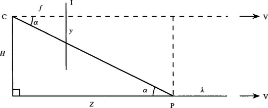
Figure 20.4 Geometry for constructing plan view of ground plane. This diagram is a vertical cross section containing the center of projection C of the camera and the vanishing point V, though vanishing point V can only be indicated by arrows. The cross section also includes a line λ within the ground plane. The projection line from a general point P on λ to the image plane I has a declination angle α, f is the focal length of the camera lens, and H is the height of the optical axis of the camera above the ground plane. Note that the optical axis of the camera is assumed to be horizontal and parallel to λ.
where Z is the distance of P along λ (Fig. 20.4), and y is the distance of the projection of P below the vanishing line in the image plane. This leads to the following value for Z:
Similar considerations lead to the lateral distance from λ being given by:
where x is the lateral distance in the image plane.
Overall, we now have related image coordinates (x, y) and world (plan view) coordinates (X, Z). Both X and Z vary rapidly with y when y is small because of the distorting (foreshortening) effects of perspective geometry. Thus, as might be expected, X and Z are more difficult to measure accurately in the distance.
More general cases are best dealt with using homogeneous coordinates that lead to linear transformations using 4 × 4 matrices (Chapter 21).
20.7 Further Factors Involved in Mobile Robot Navigation
We have moved from a simple image view that can successfully indicate a correct way forward to one in which experience of the situation is gradually built up. The first (image view) representation is restricted to providing ad hoc help, whereas the second (plan view) representation is the natural one for storing knowledge and arriving at globally optimal solutions. It is difficult to be sure which representation humans rely on. While it is apparently the first, the second is definitely invoked during conscious, deductive thought processes whenever detailed analysis of what is happening (e.g., in a maze) is undertaken. However, introspection is not a good means of finding out how humans actually carry out the other (subconscious) task. In any case, in a machine vision context, we merely need to see how to set about programming a software system to emulate the human.
It is profitable for us to explore how the navigation task can be undertaken, in the abstract case typified by a maze-running robot. Suppose first that the robot moves over the maze in a search mode, exploring the environment and mapping the allowed and forbidden areas. When a complete map has been built up, some purposive activity can be imposed. How should the robot go from its current position C to a goal position G in a minimum time? We can run the maze abstractly by applying an algorithm to form a distance function (Section 6.7), which starts at G and propagates around the maze, constrained only by the positions of the walls (Fig. 20.5). When the distance function arrives at C, the distance value is noted and the propagation algorithm is terminated. To find the optimum path, it is now only necessary to proceed downhill from C in the direction of the locally greatest gradient, until arriving at G (Kanesalingam et al., 1998). A distance function is used to ensure that the map contains information on which of several alternative routes is the shortest: if it were known that only one route would be possible, simple propagation operations of the type used in connected components analysis would be adequate for locating it.
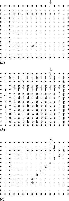
Figure 20.5 Use of distance function for path planning. (a) A rudimentary maze. (b) Distance function of the maze, with origin at the goal (marked ⊗). (c) Optimum path deduced by tracking from the entrance to the maze (marked with an arrow) along directions of maximum gradient. For convenience of display, the distance function is coded in letters, starting with a = 1. Improved forms of distance function would lead to more accurate path optimization.
Thus far we have only considered mobile robots capable of rolling or walking down corridors or paths. However, much of what has been talked about also applies to vehicles driving down city roads because perspective lines are quite common in such situations. However, it will be difficult to apply these ideas to country roads which meander along largely unpredictable paths. In such cases, the concept of a VP has to be replaced by a sequence of VPs that move along a vanishing line–typically, the horizon line (Billingsley and Schoenfisch, 1995). Although this complication does not invalidate the general technique, the straight-line detection approach becomes inappropriate, and more suitable methods must be devised. The image-based model can probably still be used for instantaneous steering–especially if a Kalman filter (Section 18.13) is used to maintain continuity. However, practical accident-free country driving will require considerably more realistic scene interpretation than analysis based simply on where the current VP might be. After all, images are rich in cues which the human is able to discern and use–by virtue of the huge database of relevant information stored in the human mind. Robot vision capabilities do not yet match up to this task with the required reliability and speed–though excellent efforts are being made. The next decade will undoubtedly see a revolution in what can be achieved.
20.8 More on Vanishing Points
The cross ratio can turn up in many situations and on each occasion provide yet another neat result. An example is when a road or pavement has flagstones whose boundaries are well demarcated and easily measurable. They can then be used to estimate the position of the vanishing point on the ground plane. Imagine viewing the flagstones obliquely from above, with the camera or the eyes aligned horizontally (Fig. 20.3b). Then we have the geometry of Fig. 20.6 where the points O, H1,H2 lie on the ground plane, while O, V1,V2,V3 are in the image plane.2
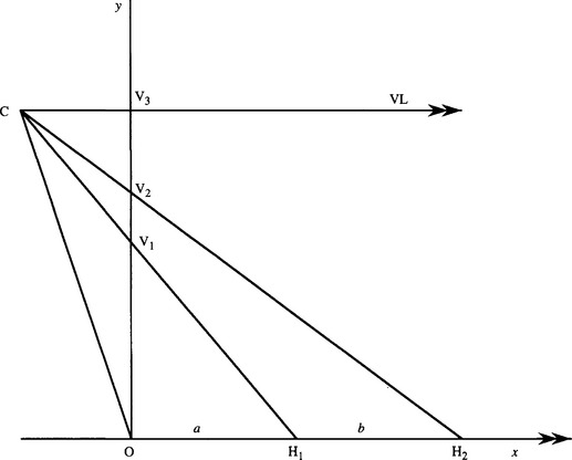
Figure 20.6 Geometry for finding the vanishing line from a known pair of spacings. C is the center of projection. VL is the vanishing line direction, which is parallel to the ground plane OH1H2. Although the camera plane OV1V2V2 is drawn perpendicular to the ground plane, this is not necessary for successful operation of the algorithm (see text).
If we regard C as a center of projection, the cross ratio formed from the points O, V1,V2,V3 must have the same value as that formed from the points O, H1,H2, and infinity in the horizontal direction. Supposing that OH1 and H1H2 have known lengths a and b, equating the cross ratio values gives:
This allows us to estimate y3:
If a = b (as is likely to be the case for flagstones):
Notice that this proof does not actually assume that points V1,V2,V3 are vertically above the origin, or that line OH1H2 is horizontal. Rather, these points are seen to lie along two coplanar straight lines, with C in the same plane. Also, note that only the ratio of a to b, not their absolute values, is relevant in this calculation.
Having found y3, we have calculated the direction of the vanishing point, whether or not the ground plane on which it lies is actually horizontal, and whether or not the camera axis is horizontal.
Finally, notice that equation (20.8) can be rewritten in the simpler form:
The inverse factors give some intuition into the processes involved–not the least of which is considering the inverse relation between distance along the ground plane and image distance from the vanishing line in equation (20.2)–and similarly, the inverse relation between depth and disparity in equation (16.5).
20.9 Centers of Circles and Ellipses
It is well known that circles and ellipses project into ellipses (or occasionally into circles). This statement is widely applicable and is valid for orthographic projection, scaled orthographic projection, weak perspective projection, and full projective projection.
Another factor that is easy to overlook is what happens to the center of the circle or ellipse under these transformations. It turns out that the ellipse (or circle) center does not project into the ellipse (or circle) center under full perspective projection; there will in general be a small offset (Fig. 20.7).3
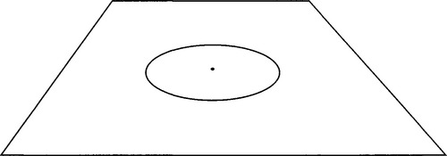
Figure 20.7 Projected position of a circle center under full perspective projection. Note that the projected center is not at the center of the ellipse in the image plane.
If the position of the vanishing line of the plane can be identified in the image, the calculation of the offset for a circle is quite simple using the theory of Section 20.8, which applies as the center of a circle bisects its diameter (Fig. 20.8). First, let ε be the shift in the center, let d be the distance of the center of the ellipse from the vanishing line, and b be the length of the semiminor axis. Next, identify b + ε with y1,2b with y2,and b + d with y3. Finally, substitute for y1, y2, and y3 in equation (20.8). We then obtain the result:
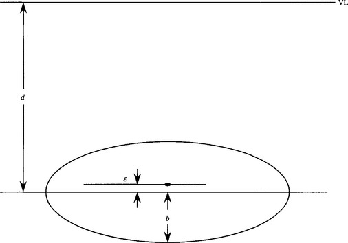
Figure 20.8 Geometry for calculating the offset of the circle center. The projected center of the circle is shown as the elongated dot, and the center of the ellipse in the image plane is a distance d below the vanishing line VL.
Notice that, unlike the situation in Section 20.8, here we are assuming that y3 is known and we are using its value to calculate y1 and hence ε.
If the vanishing line is not known, but the orientation of the plane on which the circle lies is known, as is also the orientation of the image plane, then the vanishing line can be deduced and the calculation can again proceed as above. However, this approach assumes that the camera has been calibrated (see Chapter 21).
The problem of center determination when an ellipse is projected into an ellipse is a little more difficult to solve: not only is the longitudinal position of the center unknown, but so is the lateral position. Nevertheless, the same basic projective ideas apply. Specifically, let us consider a pair of parallel tangents to the ellipse, which in the image become a pair of lines λ1, λ2 meeting on the vanishing line (Fig. 20.9). As the chord joining the contact points of the tangents passes through the center of the original ellipse, and as this property is projectively invariant, so the projected center must lie on the chord joining the contact points of the line-pair λ1, λ2. As the same applies for all pairs of parallel tangents to the original ellipse, we can straightforwardly locate the projected center of the ellipse in the image plane.4 For an alternative, numerical analysis of the situation, see Zhang and Wei (2003).
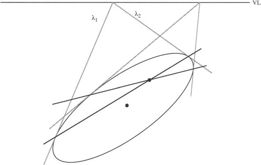
Figure 20.9 Construction for calculating the offsets for a projected ellipse. The two lines λ1,λ2 from a point on the vanishing line VL touch the ellipse, and the joins of the points of contact for all such line pairs pass through the projected center. (The figure shows just two chords of contact.)
Both the circle result and the ellipse result are important in cases of inspection of mechanical parts, where accurate results of center positions have to be made regardless of any perspective distortions that may arise. Indeed, circles can also be used for camera calibration purposes, and again high accuracy is required (Heikkilä, 2000).
20.10 Vehicle Guidance in Agriculture–A Case Study
In recent years, farmers have been increasingly pressured to reduce the quantities of chemicals they use for crop protection. This cry has come from both environmentalists and the consumers themselves. The solution to this problem lies in more selective spraying of crops. For example, it would be useful to have a machine that would recognize and spray weeds with herbicides, leaving the vegetable crops themselves unharmed. Alternatively, the individual plants could be sprayed with pesticides. This case study relates to the design of a vehicle that is capable of tracking plant rows and selecting individual plants for spraying (Marchant and Brivot, 1995; Marchant, 1996; Brivot and Marchant, 1996; Sanchiz et al., 1996; Marchant et al., 1998).5
The problem would be enormously simplified if plants grew in highly regular placement patterns, so that the machine could tell “at a glance” from their positions whether they were weeds or plants and deal with them accordingly. However, the growth of biological systems is unpredictable and renders such a simplistic approach impracticable. Nevertheless, if plants are grown from seed in a greenhouse and transplanted to the field when they are approaching 100 mm high, they can be placed in straight parallel rows, which will be approximately retained as they grow to full size. There is then the hope (as in the case shown in Fig. 2.2) that the straight rows can be extracted by relatively simple vision algorithms, and the plants themselves located and identified straightforwardly.
At this stage the problems are (1) that the plants will have grown to one side or another and will thus be out of line; (2) that some will have died; (3) that weeds will have appeared near some of the plants; and (4) that some plants will have grown too slowly, and will not be recognized as plants. Thus, a robust algorithm will be required to perform the initial search for the plant rows. The Hough transform approach is well adapted to this type of situation: specifically, it is well suited to looking for line structure in images.
The first step in the process is to locate the plants. This can be achieved with reasonable accuracy by thresholding the input images. (This process is eased if infrared wavelengths are used to enhance contrast.) At this stage, however, the plant images become shapeless blobs or clumps (Fig. 20.10). These contain holes and lobes (the leaves, in the case of cabbages or cauliflowers), but a certain amount of tidying up can be achieved either by placing a bounding box around the object shape or by performing a dilation of the shape which will regularize it and fill in the major concavities (the real-time solution employed the first of these methods). Then the position of the center of mass of the shape is determined, and it is this that is fed to the Hough transform straight-line (plant row) detector. In common with the usual Hough transform approach, votes are accumulated in parameter space for all possible parameter combinations consistent with the input data. This means taking all possible line gradients and intercepts for lines passing through a given plant center and accumulating them in parameter space. To help get the most meaningful solution, it is useful to accumulate values in proportion to the plant area. In addition, it should be noted that if three rows of plants appear in any image, it will not initially be known which plant is in which row. Therefore, each plant should be allowed to vote for all the row positions. This will naturally be possible only if the inter-row spacing is known and can be assumed in the analysis. However, if this procedure is followed, the method will be far more resistant to missing plants and to weeds that are initially mistakenly assumed to be plants.
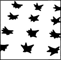
Figure 20.10 Perspective view of plant rows after thresholding. In this idealized sketch, no background clutter is shown.
The algorithm is improved by preferentially eliminating weeds from the images before applying the Hough transform. Weed elimination is achieved by three techniques: hysteresis thresholding, dilation, and blob size filtering. Dilation refers to the standard shape expansion technique described in Chapter 8 and is used here to fill in the holes in the plant blobs. Filtering by blob area is reasonable since the weeds are seldom as strong as the plants, which were transplanted only when they had become well established.
Hysteresis thresholding is a widely used technique that involves the use of two threshold levels. In this case, if the intensity is greater than the upper level tu, the object is taken to be plant, if lower than the lower level t1, it is taken to be weed; if at an intermediate level and next to a region classified as plant, it is taken to be plant. The plant region is allowed to extend sequentially as far as necessary, given only that there is a contiguous region of intensity between t1 and tu connecting a given point to a true plant (≥ tu) region. This application is unusual in that whole-object segmentation is achieved using hysteresis thresholding. The technique is used more often to help create connected object boundaries (see Section 7.1.1).
Once the Hough transform has been obtained, the parameter space has to be analyzed to find the most significant peak position. Normally, there will be no doubt as to the correct peak–even though the method of accumulation permits plants from adjacent rows to contribute to each peak. With three rows each permitted to contribute to adjacent peaks, the resultant voting patterns in parameter space are: 1,1,1,0,0; 0,1,1,1,0; 0,0,1,1,1–totaling 1,2,3,2,1–thereby making the true center position the most prominent. (Actually, the position is more complicated than this as several plants will be visible in each row, thus augmenting the central position further.) However, the situation could be erroneous if any plants are missing. It is therefore useful to help the Hough transform arrive at the true central position. This can be achieved by applying a Kalman filter (Section 18.13) to keep track of the previous central positions, and anticipate where the next one will be–thereby eliminating false solutions. This concept is taken furthest in the paper by Sanchiz et al. (1996), where all the individual plants are identified on a reliable map of the crop field and allowance is systematically made for errors from any random motions of the vehicle.
20.10.1 3-D Aspects of the Task
So far we have assumed that we are looking at simple 2-D images that represent the true 3-D situation in detail. In practice, this is not a valid assumption inasmuch as the rows of plants are being viewed obliquely and therefore appear as straight lines, though with perspective distortions that shift and rotate their positions. The full position can be worked out only if the vehicle motions are kept in mind. Vehicles rolling along the rows of plants exhibit variations in speed and are subject to roll, pitch, and yaw. The first two of these motions correspond, respectively, to rotations about horizontal axes along and perpendicular to the direction of motion. These rotations, being less relevant, are ignored here. The last rotation (yaw) is important as it corresponds to rotation about a vertical axis and affects the immediate direction of motion of the vehicle.
We now have to relate the position (X, Y, Z) of a plant in 3-D with its location (x, y) in an image. We can do so with a general translation:
together with a general rotation:
 (20.12)
 (20.13)
The lens projection formulas are also relevant:
We shall not give a full analysis here, but assuming that roll and pitch are zero, and that the heading angle (direction of motion relative to the rows of plants) is, and that this is small, we obtain a quadratic equation for ψ in terms of tx. Thus, two sets of solutions are in general possible. However, it is soon found that only one solution matches the situation, as the wrong solution is not supported by the other feature point positions. This discussion shows the complications introduced by perspective projection–even when highly restrictive assumptions can be made about the geometrical configuration (in particular, ψ being small).
20.10.2 Real-time Implementation
Finally, it was found to be possible to implement the vehicle guidance system on a single processor augmented by two special hardware units–a color classifier and a chaincoder. The chaincoder is useful for fast shape analysis following boundary tracking. The overall system was able to process the input images at a rate of 10 Hz, which is sufficient for reliable vehicle guidance. Perhaps more important, the claimed accuracy is in the region of 10 mm and 1° of angle, making the whole guidance system adequate to cope with the particular slightly constrained application considered. A later implementation (Marchant et al., 1998) did a more thorough job of segmenting the individual plants (though still not using the blob size filter), obtaining a final 5 Hz sampling rate–again fast enough for real-time application in the field. All in all, this case study demonstrates the possibility of highly accurate selective spraying of weeds, thereby significantly cutting down on the amount of herbicide needed for crops such as cabbages, cauliflower, and wheat.
20.11 Concluding Remarks
Vanishing point detection is of great importance in helping to obtain a basic understanding of the scene being viewed by the robot camera. The chapter discussed simple means for creating a plan view of the scene, to help with navigation and path planning. It was found that when the ground plane is highly structured (whether with flagstones or other artifacts), cross ratio invariants can help locate vanishing points and provide additional understanding. A case study of vehicle guidance in agriculture was helpful in revealing many more practicalities about motion control.
This chapter has helped focus on mechanistic applications of machine vision and at the same time demonstrated various theoretical aspects of the subject. The circle and ellipse center location ideas of Section 20.9 are a byproduct of the theory and are presented here mainly for convenience and to demonstrate the generality of the concepts.
Egomotion is well mediated by vision, though the problems of 3-D, including perspective, are immense. This chapter has shown how judicious attention to vanishing points can provide a computationally efficient key to solving some of the practical problems. Nevertheless, motion parameters such as roll, pitch, and yaw can make life difficult in a real-time environment.
20.12 Bibliographical and Historical Notes
Mobile robots and the need for path planning are discussed by Kanesalingam et al. (1998) and by Kortenkamp et al. (1998); more recently, DeSouza and Kak (2002) have carried out a survey on vision for mobile robot navigation; see also Davison and Murray (2002). It is interesting how often vanishing point determination has been considered both in relation to egomotion for mobile robots (Lebègue and Aggarwal, 1993; Shuster et al., 1993), and in general, to the vision methodology (Magee and Aggarwal, 1984; Shufelt, 1999; Almansa et al., 2003), which is prone to suffer from inaccuracy when real off-camera data are used in any context. The seminal paper that gave rise to the crucial Gaussian sphere technique was that by Barnard (1983).
Guidance of outdoor vehicles, particularly on roads, has been discussed by a large number of authors over a period of many years. Most recently, there has been quite an explosive expansion in this area (Bertozzi and Broggi, 1998; Guiducci, 1999; Kang and Jung, 2003; Kastrinaki et al., 2003). De la Escalara et al. (2003) have extended the discussion to recognition of traffic signs. Zhou et al. (2003) have considered the situation for elderly pedestrians–though such work could also be relevant for blind people or wheelchair users. Hofmann et al. (2003) have shown that vision and radar can profitably be used together to combine the excellent spatial resolution of vision with the accurate range resolution of radar. The volume edited by Blake and Yuille (1992) provides a set of key readings on active vision.
Finally, Clark and Mirmehdi (2000, 2002) provide an interesting twist; they show how text in documents can be oriented using vanishing points. This work demonstrates that the techniques described in a volume such as the present one can never be presented in a completely logical order, for the techniques are surprisingly general. Indeed, the very purpose of such works is to emphasize what is generic so that future workers can benefit most.
20.13 Problems
1. Draw diagrams corresponding to Fig. 20.4 showing the geometry for the lateral distance from the line λ Prove equation (20.3) and state any assumptions that have to be made in the proof.
2. Redraw Fig. 20.9 using vanishing points aligned along the observed ellipse axes. Show that the problem of finding the transformed center location now reduces to two 1-D cases and that equation (20.10) can be used to obtain the transformed center coordinates.
3. A robot is walking along a path paved with rectangular flagstones. It is able to rotate its camera head so that one set of flagstone lines appears parallel while the other set converges toward a vanishing point. Show that the robot can calculate the position of the vanishing point in two ways: (1) by measuring the varying widths of individual flagstones or (2) by measuring the lengths of adjacent flagstones and proceeding according to equation (20.8). In case (1), obtain a formula that could be used to determine the position of the vanishing point. Which is the more general approach? Which would be applicable if the flagstones appeared in a flower garden in random locations and orientations?
1 Although some may consider egomotion to be a synonym for navigation, we interpret the term more widely to include both awareness plus control of motion and navigation per se. Indeed, the need to be sure of remaining upright must be part of the task of egomotion; it hardly falls into the category of navigation.
2 Notice that slightly oblique measurement of the flagstone, along a line that is not parallel to the sides of the flagstones, still permits the same cross ratio value to be obtained, as the same angular factor applies to all distances along the line.
3 The fact that this happens may perhaps suggest that ellipses will be slightly distorted under projection. There is definitely no such distortion, and the source of the shift in the center is merely that full perspective projection does not preserve length ratios–and in particular midpoints do not remain midpoints.
4 Students familiar with projective geomentry will be able to relate this to the “pole-polar” construction for a conic. In this case, the polar line is the vanishing line, and its pole is the projected center. In general, the pole is not at the center of an ellipse and will not be so unless the polar is at infinite distance. From this point of view, equation (20.9) can be understood in terms of “harmonic ranges,” y2 being the “harmonic mean” of y1 and y3.
5 Many of the details of this work are remarkably similar to those for the totally independent project undertaken in Australia by Billingsley and Schoenfisch (1995).