24.1 Introduction

The earlier chapters of this book have concentrated on interpreting images on the basis that when suitable cues have been found, the positions of various objects and their identities will emerge in a natural and straightforward way. When the objects that appear in an image have simple shapes, just one stage of processing may be required—as in the case of circular washers on a conveyor. For more complex objects, location requires at least two stages—as when graph matching methods are used. For situations where the full complexity of three dimensions occurs, more subtle procedures are usually required, as has already been seen in Chapter 16. The very ambiguity involved in interpreting the 2-D images from a set of 3-D objects generally requires cues to be sought and hypotheses to be made before any serious attempt can be made at the task. Thus, cues are vital to keying into the complex data structures of many images. For simpler situations, however, concentration on small features is valuable in permitting image interpretation to be carried out efficiently and rapidly. Neither must it be forgotten that in many applications of machine vision the task is made simpler by the fact that the main interest lies in specific types of objects; for example, the widgets to be inspected on a widget line.

The fact that it is often expedient to start by searching for cues means that the vision system could lock on to erroneous interpretations. For example, Hough-based methods lead to interpretations based on the most prominent peaks in parameter space, and the maximal clique approach supports interpretations based on the largest number of feature matches between parts of an image and the object model. Noise, background clutter, and other artifacts make it possible that an object will be seen (or its presence hypothesized) when none is there, while occlusions, shadows, and so on, may cause an object to be missed altogether.

A rigorous interpretation strategy would ideally attempt to find all possible feature and object matches and should have some means of distinguishing between them. One should not be satisfied with an interpretation until the whole of any image has been understood. However, enough has been seen in previous chapters (e.g., Chapter 11) to demonstrate that the computational load of such a strategy generally makes it impracticable, at least for real (e.g., outdoor) scenes. Yet in some more constrained situations the strategy is worth considering and various possible solutions can be evaluated carefully before a final interpretation is reached. These situations arise practically where small relevant parts of images can be segmented and interpreted in isolation. One such case is that of optical character recognition (OCR), which is commonly addressed through statistical pattern recognition (SPR).

The following sections study some of the important principles of SPR. A complete description of all the work that has been carried out in this area would take several volumes to cover. Fortunately, SPR has been researched for well over three decades and has settled down sufficiently so that an overview chapter can serve a useful purpose. The reader is referred to several existing excellent texts for further details (Duda et al., 2001; Webb, 2002). We start by describing the nearest neighbor approach to SPR and then consider Bayes’ decision theory, which provides a more general model of the underlying process.

24.2 The Nearest Neighbor Algorithm

The principle of the nearest neighbor (NN) algorithm is that of comparing input image¹ patterns against a number of paradigms and then classifying the input pattern according to the class of the paradigm that gives the closest match (Fig. 24.1). An instructive but rather trivial example is that shown in Here a number of binary patterns are presented to the computer in the training phase of the algorithm. Then the test patterns are presented one at a time and compared bit by bit against each of the training patterns. This approach yields a generally reasonable result, the main problems arising when (1) training patterns of different classes are close together in Hamming distance (i.e., they differ in too few bits to be readily distinguishable), and (2) minor translations, rotations, or noise cause variations that inhibit accurate recognition. More generally, problem (2) means that the training patterns are insufficiently representative of what will appear during the test phase. The latter statement encapsulates an exceptionally important principle and implies that there must be sufficient patterns in the training set for the algorithm to be able to generalize over all possible patterns of each class. However, problem (1) implies that patterns of two different classes may sometimes be so close as to be indistinguishable by any algorithm, and then it is inevitable that erroneous classifications will be made. As seen later in this chapter, this is because the underlying distributions in feature space overlap.

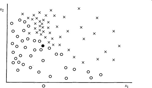
Figure 24.1 Principle of the nearest neighbor algorithm for a two-class problem: , class 1 training set patterns; ×, class 2 training set patterns; •, test pattern.

The example of Fig. 1.1 is rather trivial but nevertheless carries important lessons. General images have many more pixels than those in Fig. 1.1 and also are not merely binary. However, since it is pertinent to simplify the data as far as possible to save computation, it is usual to concentrate on various features of a typical image and classify on the basis of these. One example is provided by a more realistic version of the OCR problem where characters have linear dimensions of at least 32 pixels (although we continue to assume that the characters have been located reasonably accurately so that it remains only to classify the subimages containing them). We can start by thinning the characters to their skeletons and making measurements on the skeleton nodes and limbs (see also Chapters 1 and 6). We then obtain the numbers of nodes and limbs of various types, the lengths and relative orientations of limbs, and perhaps information on curvatures of limbs. Thus, we arrive at a set of numerical features that describe the character in the subimage.

The general technique is to plot the characters in the training set in a multidimensional feature space and to tag the plots with the classification index. Then test patterns are placed in turn in the feature space and classified according to the class of the nearest training set pattern. In this way, we generalize the method adopted in Fig. 24.1. Note that in the general case the distance in feature space is no longer Hamming distance but a more general measure such as Mahalanobis distance (Duda et al., 2001). A problem arises since there is no reason why the different dimensions in feature space should contribute equally to distance. Rather, they should each have different weights in order to match the physical problem more closely. The problem of weighting cannot be discussed in detail here, and the reader is referred to other texts such as that by Duda et al. (2001). Suffice it to say that with an appropriate definition of distance, the generalization of the method outlined here is adequate to cope with a variety of problems.

In order to achieve a suitably low error rate, large numbers of training set patterns are normally required, leading to significant storage and computation problems. Means have been found for reducing these problems through several important strategies. Notable among these strategies is that of pruning the training set by eliminating patterns which are not near the boundaries of class regions in feature space, since such patterns do not materially help reduce the misclassification rate.

An alternative strategy for obtaining equivalent performance at lower computational cost is to employ a piecewise linear or other functional classifier instead of the original training set. It will be clear that the NN method itself can be replaced, with no change in performance, by a set of planar decision surfaces that are the perpendicular bisectors (or their analogs in multidimensional space) of the lines joining pairs of training patterns of different classes that are on the boundaries of class regions. If this system of planar surfaces is simplified by any convenient means, then the computational load may be reduced further (Fig. 24.2). This may be achieved either indirectly by some smoothing process or directly by finding training procedures that act to update the positions of decision surfaces immediately on receipt of each new training set pattern. The second approach is in many ways more attractive than the first since it drastically cuts down storage requirements—although it must be confirmed that a training procedure is selected which converges sufficiently rapidly. Again, discussion of this well-researched topic is left to other texts (Nilsson, 1965; Duda et al., 2001; Webb, 2002).

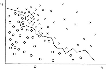
Figure 24.2 Use of planar decision surfaces for pattern classification. In this example the “planar decision surface” reduces to a piecewise linear decision boundary in two dimensions. Once the decision boundary is known, the training set patterns themselves need no longer be stored.

We now turn to a more generalized approach—Bayes’ decision theory which underpins all the possibilities created by the NN method and its derivatives.

24.3 Bayes’ Decision Theory

The basis of Bayes’ decision theory will now be examined. To get a computer to classify objects, we need to measure some prominent feature of each object such as its length and to use this feature as an aid to classification. Sometimes such a feature may give very little indication of the pattern class—perhaps because of the effects of manufacturing variation. For example, a handwritten character may be so ill formed that its features are of little help in interpreting it. It then becomes much more reliable to make use of the known relative frequencies of letters, or to invoke context: in fact, either of these strategies can give a greatly increased probability of correct interpretation. In other words, when feature measurements are found to be giving an error rate above a certain threshold, it is more reliable to employ the a priori probability of a given pattern appearing.

The next step in improving recognition performance is to combine the information from feature measurements and from a priori probabilities by applying Bayes’ rule. For a single feature x this takes the form:

     (24.1)

where

     (24.2)

Mathematically, the variables here are (1) the a priori probability of class C_i, P(C_i); (2) the probability density for feature x, p(x); (3) the class-conditional probability density for feature x in class C_i, p(x|C_i)—that is, the probability that feature x arises for objects known to be in class C_i; and (4) the a posteriori probability of class C_i when x is observed, P(C_i|x).

The notation P(C_i|x) is by now a standard one, being defined as the probability that the class is C_i when the feature is known to have the value x. Bayes’ rule now says that to find the class of an object we need to know two sets of information about the objects that might be viewed. The first set is the basic probability P(C_i) that a particular class might arise; the second is the distribution of values of the feature x for each class. Fortunately, each of these sets of information can be found straightforwardly by observing a sequence of objects, for example, as they move along a conveyor. Such a sequence of objects is again called the training set.

Many common image analysis techniques give features that may be used to help identify or classify objects. These include the area of an object, its perimeter, the numbers of holes it possesses, and so on. Classification performance may be improved not only by making use of the a priori probability but also by employing a number of features simultaneously. Generally, increasing the number of features helps to resolve object classes and reduce classification errors (Fig. 24.3). However, the error rate is rarely reduced to zero merely by adding more and more features, and indeed the situation eventually deteriorates for reasons explained in Section 24.5.

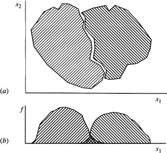
Figure 24.3 Use of several features to reduce classification errors: (a) the two regions to be separated in 2-D (x₁, x₂) feature space; (b) frequencies of occurrence of the two classes when the pattern vectors are projected onto the x₁-axis. Error rates will be high when either feature is used on its own but will be reduced to a low level when both features are employed together.

Bayes’ rule can be generalized to cover the case of a generalized feature x, in multidimensional feature space, by using the modified formula:

     (24.3)

where P(C_i) is the a priori probability of class C_i, and p(x) is the overall probability density for feature vector x:

     (24.4)

The classification procedure is then to compare the values of all the P(C_j |x) and to classify an object as class C_i if:

     (24.5)

24.4 Relation of the Nearest Neighbor and Bayes’ Approaches

When Bayes’ theory is applied to simple pattern recognition tasks, it is immediately clear that a priori probabilities are important in determining the final classification of any pattern, since these probabilities arise explicitly in the calculation. However, this is not so for the NN type of classifier. The whole idea of the NN classifier appears to be to get away from such considerations, instead classifying patterns on the basis of training set patterns that lie nearby in feature space. However, there must be a definite answer to the question of whether or not a priori probabilities are taken into account implicitly in the NN formulation, and therefore of whether or not an adjustment needs to be made to the NN classifier to minimize the error rate. Since a categorical statement of the situation is important the next subsection provides such a statement, together with necessary analysis.

24.5 The Optimum Number of Features

Section 24.3 stated that error rates can be reduced by increasing the number of features used by a classifier, but there is a limit to this, after which performance actually deteriorates. In this section we consider why this should happen. Basically, the reason is similar to the situation where many parameters are used to fit a curve to a set of D data points. As the number of parameters P is increased, the fit of the curve becomes better and better, and in general becomes perfect when P = D. However, by that stage the significance of the fit is poor, since the parameters are no longer overdetermined and no averaging of their values is taking place. Essentially, all the noise in the raw input data is being transferred to the parameters. The same thing happens with training set patterns in feature space. Eventually, training set patterns are so sparsely packed in feature space that the test patterns have reduced the probability of being nearest to a pattern of the same class, so error rates become very high. This situation can also be regarded as due to a proportion of the features having negligible statistical significances; that is, they add little additional information and serve merely to add uncertainty to the system.

However, an important factor is that the optimum number of features depends on the amount of training a classifier receives. If the number of training set patterns is increased, more evidence is available to support the determination of a greater number of features and hence to provide more accurate classification of test patterns. In the limit of very large numbers of training set patterns, performance continues to increase as the number of features is increased.

This situation was first clarified by Hughes (1968) and verified in the case of n-tuple pattern recognition—a variant of the NN classifier due to Bledsoe and Browning (1959)—by Ullmann (1969). Both workers produced clear curves showing the initial improvement in classifier performance as the number of features increased; this improvement was followed by reduced performance for large numbers of features.

Before leaving this topic, note that the above arguments relate to the number of features that should be used but not to their selection. Some features are more significant than others, the situation being very data-dependent. We will leave it as a topic for experimental tests to determine which subset of features will minimize classification errors (see also Chittineni, 1980).

24.6 Cost Functions and the Error–Reject Tradeoff

The forgoing sections implied that the main criterion for correct classification is that of maximum a posteriori probability. Although probability is always a relevant factor, in a practical engineering environment it is often more important to minimize costs. Hence, it is necessary to compare the costs involved in making correct or incorrect decisions. Such considerations can be expressed mathematically by invoking a loss function L(C_i|C_j) that represents the cost involved in making a decision C_i when the true class for feature x is C_j.

To find a modified decision rule based on minimizing costs, we first define a function known as the conditional risk:

     (24.13)

This function expresses the expected cost of deciding on class C_I when x is observed. In order to minimize this function, we now decide on class C_I only if:

     (24.14)

If we were to choose a particularly simple cost function, of the form:

     (24.15)

then the result would turn out to be identical to the previous probability-based decision rule, relation (24.5). Only when certain errors lead to relatively large (or small) costs does it pay to deviate from the normal decision rule. Such cases arise when we are in a hostile environment and must, for example, give precedence to the sound of an enemy tank over that of other vehicles. It is better to be oversensitive and risk a false alarm than to chance not noticing the hostile agent. Similarly, on a production line it may sometimes be better to reject a small number of good products than to risk selling a defective product. Cost functions therefore permit classifications to be biased in favor of a safe decision in a rigorous, predetermined, and controlled manner, and the desired balance of properties obtained from the classifier.

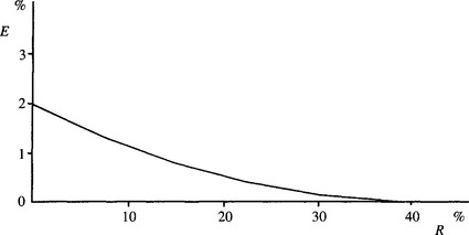
Another way of minimizing costs is to arrange for the classifier to recognize when it is “doubtful” about a particular classification because two or more classes are almost equally likely. Then one solution is to make a safe decision, the decision plane in feature space being biased away from its position for maximum probability classification. An alternative is to reject the pattern, that is, place it into an “unknown” category. In that case, some other means can be employed for making an appropriate classification. Such a classification could be made by going back to the original data and measuring further features, but in many cases it is more appropriate for a human operator to be available to make the final decision. The latter approach is more expensive, and so introducing a “reject” classification can incur a relatively large cost factor. A further problem is that the error rate² is reduced only by a fraction of the amount that the rejection rate is increased. In a simple two-class system, the initial decrease in error rate is only one-half the initial increase in reject rate (i.e., a 1% decrease in error rate is obtained only at the expense of a 2% increase in reject rate); the situation gets rapidly worse as progressively lower error rates are attempted (Fig. 24.4). Thus, very careful cost analysis of the error–reject tradeoff curve must be made before an optimal scheme can be developed. Finally, it should be noted that the overall error rate of the classification system depends on the error rate of the classifier that examines the rejects (e.g., the human operator); this consideration needs to be taken into account in determining the exact tradeoff to be used.

Figure 24.4 An error-reject tradeoff curve (E, error rate; R, reject rate). In this example, the error rate E drops substantially to zero for a reject rate R of 40%. More usually, E cannot be reduced to zero until R is 100%.

24.7 The Receiver–Operator Characteristic

The early sections of this chapter suggest an implicit understanding that classification error rates have to be reduced as far as possible, though in the last section it was acknowledged that it is cost rather than error that is the practically important parameter. It was also found that a tradeoff between error rate and reject rate allows a further refinement to be made to the analysis.

Here we consider another refinement that is required in many practical cases where binary decisions have to be made. Radar provides a good illustration showing that there are two basic types of misclassifications: (1) radar displays may indicate an aircraft or missile when none is present—in which case the error is called a false positive (or in popular parlance, a false alarm); (2) radar may indicate that no aircraft or missile is present when there actually is one—in which case the error is called a false negative. Similarly, in automated industrial inspection, when searching for deficient products, a false positive corresponds to finding one when none is present, whereas a false negative corresponds to missing a deficient product when one is present.

There are four relevant categories: (1) true positives (positives that are correctly classified), (2) true negatives (negatives that are correctly classified), (3) false positives (positives that are incorrectly classified), and (4) false negatives (negatives that are incorrectly classified). If many experiments are carried out to determine the proportions of these four categories in a given application, we can obtain the four probabilities of occurrence. Using an obvious notation, we can relate these categories by the following formulas:

     (24.16)

     (24.17)

(In case the reader finds the combinations of probabilities in these formulas confusing, it is worth noting that an object that is actually a faulty product will either be correctly detected as such or else it will be incorrectly categorized as acceptable—in which case it is a false negative.)

It will be apparent that the probability of error P_E is the sum:

     (24.18)

In general, false positives and false negatives will have different costs. Thus, the loss function L(C₁|C₂) will not be the same as the loss function L(C₂|C₁). For example, missing an enemy missile or failing to find a glass splinter in baby food may be far more costly than the cost of a few false alarms (which in the case of food inspection merely means the rejection of a few good products). In many applications, there is a prime need to reduce as far as possible the number of false negatives (the number of failures to detect the requisite targets).

But how far should we go to reduce the number of false negatives? This question is an important one that should be answered by systematic analysis rather than by ad hoc procedures. The key to achieving this is to note that the proportions of false positives and false negatives will vary independently with the system setup parameters, though frequently only a single threshold parameter need be considered in any detail. In that case, we can eliminate this parameter and determine how the numbers of false positives and false negatives depend on each other. The result is the receiver–operator characteristic or ROC curve (Fig. 24.5).³

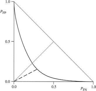
Figure 24.5 Idealized ROC curve. The gray line of gradient +1 indicates the position which a priori might be expected to lead to minimum error. The optimum working point is that indicated by the dotted line, where the gradient on the curve is − 1. The gray line of gradient −1 indicates the limiting worst case scenario. All practical ROC curves will lie below this line.

The ROC curve will often be approximately symmetrical, and, if expressed in terms of probabilities rather than numbers of items, will pass through the points (1, 0), (0, 1), as shown in Fig. 24.5. It will generally be highly concave, so it will pass well below the line P_FP + P_FN = 1, except at its two ends. The point closest to the origin will often be close to the line P_FP = P_FN. Thus, if false positives and false negatives are assigned equal costs, the classifier can be optimized simply by minimizing P_E with the constraint P_FP = P_FN. Note, however, that in general the point closest to the origin is not the point that minimizes P_E; the point that minimizes total error is actually the point on the ROC curve where the gradient is −1 (Fig. 24.5).

Unfortunately, no general theory can predict the shape of the ROC curve. Furthermore, the number of samples in the training set may be limited (especially in inspection if rare contaminants are being sought), and then it may not prove possible to make an accurate assessment of the shape—especially in the extreme wings of the curve. In some cases, this problem can be handled by modeling, for example, using exponential or other functions—as shown in Fig. 24.6, where the exponential functions lead to reasonably accurate descriptions. However, the underlying shape can hardly be exactly exponential, for this would suggest that the ROC curve tends to zero at infinity rather than at the points (1, 0), (0, 1). Also, there will in principle be a continuity problem at the join of two exponentials. Nevertheless, if the model is reasonably accurate over a good range of thresholds, the relative cost factors for false positives and false negatives can be adjusted appropriately and an ideal working point can be determined systematically. Of course, there may be other considerations: for example, it may not be permissible for the false negative rate to rise above a certain critical level. For examples of the use of the ROC analysis, see Keagy et al. (1995, 1996) and Davies et al. (2003c).

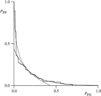
Figure 24.6 Fitting an ROC curve using exponential functions. Here the given ROC curve (see Davies et al., 2003) has distinctive steps resulting from a limited set of data points. A pair of exponential curves fits the ROC curve quite well along the two axes, each having an obvious region that it models best. In this case, the crossover region is reasonably smooth, but there is no real theoretical reason for this. Furthermore, exponential functions will not pass through the limiting points (0, 1) and (1, 0).

24.8 Multiple Classifiers

In recent years, moves have been initiated to make the classification process more reliable by application of multiple classifiers working in cooperation. The basic concept is much like that of three magistrates coming together to make a more reliable judgment than any can make alone. Each is expert in a variety of things, but not in everything, so putting their knowledge together in an appropriate way should permit more reliable judgments to be made. A similar concept applies to expert AI systems. Multiple expert systems should be able to make up for each other’s shortcomings. In all these cases, some way should exist to get the most out of the individual classifiers without confusion reigning.

The idea is not just to take all the feature detectors that the classifiers use and to replace their output decision-making devices with a single more complex decision-making unit. Indeed, such a strategy could well run into the problem discussed in Section 24.5—of exceeding the optimum number of features. At best only a minor improvement would result from such a strategy, and at worst the system would be grossly failure-prone. On the contrary, the idea is to take the final classification of a number of complete but totally separate classifiers and to combine their outputs to obtain a substantially improved output. Furthermore, the separate classifiers might use totally different strategies to arrive at their decisions. One may be a nearest neighbor classifier, another may be a Bayes classifier, and yet another may be a neural network classifier (see Chapter 25). Similarly, one might employ structural pattern recognition, another might use statistical pattern recognition, and yet another might use syntactic pattern recognition. Each will be respectable in its own right: each will have strengths, but each will also have weaknesses. Part of the idea is one of convenience: to make use of any soundly based classifier that is available, and to boost its effectiveness by using it in conjunction with other soundly based classifiers.

The next task is to determine how this can be achieved in practice. Perhaps the most obvious way forward is to get the individual classifiers to vote for the class of each input pattern. Although this is a nice idea, it will often fail because the individual classifiers may have more weaknesses than strengths. At the very least, the concept must be made more sophisticated.

Another strategy is again to allow the individual classifiers to vote but this time to make them do so in an exclusive manner, so that as many classes as possible are eliminated for each input pattern. This objective is achievable with a simple intersection rule: a class is accepted as a possibility only if all the classifiers indicate that it is a possibility. The strategy is implemented by applying a threshold to each classifier in a special way, which will now be described.

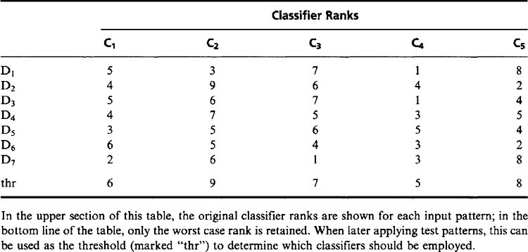
A prerequisite for this strategy to work is that each classifier must give not only a class decision for each input pattern but also the ranks of all possible classes for each pattern. In other words, it must give its first choice of class for any pattern, its second choice for that pattern, and so on. Then the classifier is labeled with the rank it assigned to the true class of that pattern. We apply each classifier to the whole training set and get a table of ranks (Table 24.1). Finally, we find the worst case (largest rank)⁴ for each classifier, and we take that as a threshold value that will be used in the final multiple classifier. When using this method for testing input patterns, only those classifiers that are not excluded by the threshold have their outputs intersected to give the final list of classes for the input pattern.

Table 24.1 Determining a set of classifiers for the intersection strategy

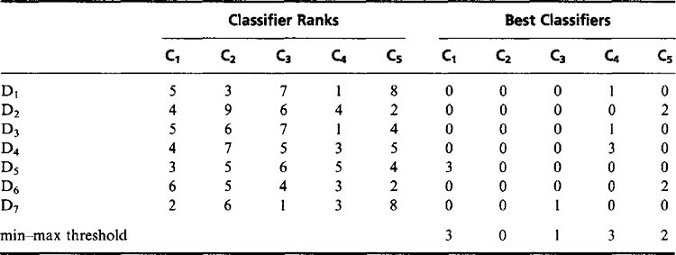
This “intersection strategy” focuses on the worst-case behavior of the individual classifiers, and the result could be that a number of classifiers will hardly reduce the list of possible classes for the input patterns. This tendency can be tackled by an alternative union strategy, which focuses on the specialisms of the individual classifiers. The aim is then to find a classifier that recognizes each particular pattern well. To achieve this we look for the classifier with the smallest rank (classifier rank being defined exactly as already defined above for the intersection strategy) for each individual pattern (Table 24.2). Having found the smallest rank for the individual input patterns, we determine the largest of these ranks that arises for each classifier as we go right through all the input patterns. Applying this value as a threshold now determines whether the output of the classifier should be used to help determine the class of a pattern. Note that the threshold is determined in this way using the training set and is later used to decide which classifiers to apply to individual test patterns. Thus, for any pattern a restricted set of classifiers is identified that can best judge its class.

Table 24.2 Determining a set of classifiers for the union strategy

To clarify the operation of the union strategy, let us examine how well it will work on the training set. It is guaranteed to retain enough classifiers to ensure that the true class of any pattern is not excluded (though naturally this is not guaranteed for any member of the test set). Hence, the aim of employing a classifier that recognizes each particular pattern well is definitely achieved.

Unfortunately, this guarantee is not obtained without cost. Specifically, if a member of the training set is actually an outlier, the guarantee will still apply, and the overall performance may be compromised. This problem can be addressed in many ways, but a simple possibility is to eliminate excessively bad exemplars from the training set. Another way is to abandon the union strategy altogether and go for a more sophisticated voting strategy. Other approaches involve reordering the data to improve the rank of the correct class (Ho et al., 1994).

24.9 Cluster Analysis

24.9.1 Supervised and Unsupervised Learning

In the earlier parts of this chapter, we made the implicit assumption that the classes of all the training set patterns are known, and in addition that they should be used in training the classifier. Although this assumption might be regarded as inescapable, classifiers may actually use two approaches to learning—supervised learning (in which the classes are known and used in training) and unsupervised learning (in which they are either unknown or known and not used in training). Unsupervised learning can frequently be advantageous in practical situations. For example, a human operator is not required to label all the products coming along a conveyor, as the computer can find out for itself both how many classes of product there are and which categories they fall into. In this way, considerable operator effort is eliminated. In addition, it is not unlikely that a number of errors would thereby be circumvented. Unfortunately, unsupervised learning involves a number of difficulties, as will be seen in the following subsections.

Before proceeding, we should state two other reasons why unsupervised learning is useful. First, when the characteristics of objects vary with time—for example, beans changing in size and color as the season develops—it will be necessary to track these characteristics within the classifier. Unsupervised learning provides an excellent means of approaching this task. Second, when setting up a recognition system, the characteristics of objects, and in particular their most important parameters (e.g., from the point of view of quality control) may well be unknown, and it will be useful to gain some insight into the nature of the data. Thus, types of faults will need to be logged, and permissible variants on objects will need to be noted. As an example, many OCR fonts (such as Times Roman) have a letter “a” with a stroke bent over the top from right to left, though other fonts (such as Monaco) do not have this feature. An unsupervised classifier will be able to flag this difference by locating a cluster of training set patterns in a totally separate part of feature space (see Fig. 24.7). In general, unsupervised learning is about the location of clusters in feature space.

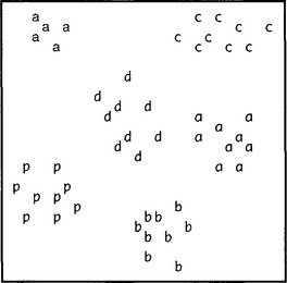
Figure 24.7 Location of clusters in feature space. Here the letters correspond to samples of characters taken from various fonts. The small cluster of a’s with strokes bent over the top from right to left appear at a separate location in feature space. This type of deviation should be detectable by cluster analysis.

24.9.2 Clustering Procedures

As we have said, an important reason for performing cluster analysis is characterization of the input data. However, the underlying motivation is normally to classify test data patterns reliably. To achieve these aims, it will be necessary both to partition feature space into regions corresponding to significant clusters and to label each region (and cluster) according to the types of data involved. In practice, this can happen in two ways:

1. By performing cluster analysis and then labeling the clusters by specific queries to human operators on the classes of a small number of individual training set patterns.

2. By performing supervised learning on a small number of training set patterns and then performing unsupervised learning to expand the training set to realistic numbers of examples.

In either case, we see that ultimately we do not escape from the need for supervised classification. However, by placing the main emphasis on unsupervised learning, we reduce the tedium and help prevent preconceived ideas on possible classes from affecting the final recognition performance.

Before proceeding further, we should note in some cases we may have absolutely no idea in advance about the number of clusters in feature space. This occurs in classifying the various regions in satellite images. Such cases are in direct contrast with applications such as OCR or recognizing chocolates being placed in a chocolate box.

Unfortunately, cluster analysis involves some very significant problems. Not least is the visualization problem. First, in one, two, or even three dimensions, we can easily visualize and decide on the number and location of any clusters, but this capability is misleading. We cannot extend this capability to feature spaces of many dimensions. Second, computers do not visualize as we do, and special algorithms will have to be provided to enable them to do so. Now computers could be made to emulate our capability in low-dimensional feature spaces, but a combinatorial explosion would occur if we attempted this for high-dimensional spaces. We will therefore have to develop algorithms that operate on lists of feature vectors, if we are to produce automatic procedures for cluster location.

Available algorithms for cluster analysis fall into two main groups—agglomerative and divisive. Agglomerative algorithms start by taking the individual feature points (training set patterns, excluding class) and progressively grouping them together according to some similarity function until a suitable target criterion is reached. Divisive algorithms start by taking the whole set of feature points as a single large cluster and progressively dividing it until some suitable target criterion is reached. Let us assume that there are P feature points. Then, in the worst case, the number of comparisons between pairs of individual feature point positions that will be required to decide whether to combine a pair of clusters in an agglomerative algorithm will be:

     (24.19)

while the number of iterations required to complete the process will be of order P–k. (Here we are assuming that the final number of clusters to be found is k, where k ≤ P.) On the other hand, for a divisive algorithm, the number of comparisons between pairs of individual feature point positions will be reduced to:

     (24.20)

while the number of iterations required to complete the process will be of order k.

Although it would appear that divisive algorithms require far less computation than agglomerative algorithms, this is not so. This is because any cluster containing p feature points will have to be examined for a huge number of potential splits into subclusters, the actual number being of the order:

     (24.21)

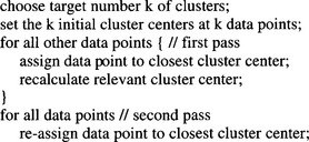
In general, the agglomerative approach will have to be adopted. In fact, the type of agglomerative approach outlined above is exhaustive and rigorous, and a less exacting, iterative approach can be used. First, a suitable number k of cluster centers are set. (These can be decided from a priori considerations or by making arbitrary choices.) Second, each feature vector is assigned to the closest cluster center. Third, the cluster centers are recalculated. This process is repeated if any feature points have moved from one cluster to another during the iteration, though termination can also be instituted if the quality of clustering ceases to improve. The overall algorithm, which was originally due to Forgy (1965), is given in Fig. 24.8.

Figure 24.8 Basis of Forgy’s algorithm for cluster analysis.

The effectiveness of this algorithm will be highly data-dependent, in particular with regard to the order in which the data points are presented. In addition, the result could be oscillatory or nonoptimal (in the sense of not arriving at the best solution). This could happen if at any stage a single cluster center arose near the center of a pair of small clusters. In addition, the method gives no indication of the most appropriate number of clusters. Accordingly, a number of variant and alternative algorithms have been devised. One such algorithm is the ISODATA algorithm (Ball and Hall, 1966). This is similar to Forgy’s method but is able to merge clusters that are close together and to split elongated clusters.

Another disadvantage of iterative algorithms is that it may not be obvious when to get them to terminate. As a result, they are liable to be too computation intensive. Thus, there has been some support for noniterative algorithms. MacQueen’s k-means algorithm (MacQueen, 1967) is one of the best known noniterative clustering algorithms. It involves two runs over the data points, one being required to find the cluster centers and the other being required to finally classify the patterns (see Fig. 24.9). Again, the choice of which data points are to act as the initial cluster centers can be either arbitrary or made on some more informed basis.

Figure 24.9 Basis of MacQueen’s k-means algorithm.

Noniterative algorithms are, as indicated earlier, largely dependent on the order of presentation of the data points. With image data this is especially problematic, as the first few data points are quite likely to be similar (e.g., all derived from sky or other background pixels). A useful way of overcoming this problem is to randomize the choice of data points, so that they can arise from anywhere in the image. In general, noniterative clustering algorithms are less effective than iterative algorithms because they are overinfluenced by the order of presentation of the data.

Overall, the main problem with the algorithms described above is the lack of indication they give of the most appropriate value of k. However, if a range of possible values for k is known, all of them can be tried (using one of the above algorithms), and the one giving the best performance in respect to some suitable target criterion can be taken as providing an optimal result. In that case, we will have found the set of clusters which, in some specified sense, gives the best overall description of the data. Alternatively, some method of analyzing the data to determine k can be used before final cluster analysis, for example, using the k-means algorithm; the Zhang and Modestino (1990) approach falls into this category.

24.10 Principal Components Analysis

Closely related to cluster analysis is the concept of data representation. One powerful way of approaching this task is that of principal components analysis. This approach involves finding the mean of a cluster of points in feature space and then finding the principal axes of the cluster in the following way. First an axis is found that passes through the mean position and which gives the maximum variance when the data are projected onto it. Then a second such axis is found which maximizes variance in a direction normal to the first. This process is carried out until a total of N principal axes have been found for an N-dimensional feature space. The process is illustrated in Fig. 24.10. The process is entirely mathematical and need not be undertaken in the strict sequence indicated here. It merely involves finding a set of orthogonal axes that diagonalize the covariance matrix.

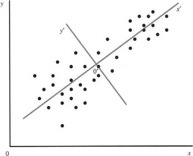
Figure 24.10 Illustration of principal components analysis. Here the dots represent patterns in feature space and are initially measured relative to the x- and y-axes. Then the sample mean is located at 0′, and the direction 0′x′ of the first principal component is found as the direction along which the variance is maximized. The direction 0′y′ of the second principal component is normal to 0′x′ in a higher dimensional space, it would be found as the direction normal to 0 x along which the variance is maximized.

The covariance matrix for the input population is defined as:

     (24.22)

where x(_p) is the location of the pth data point, m is the mean of the P data points, and E{…} indicates expectation value for the underlying population. We can estimate C from the equations:

     (24.23)

     (24.24)

Since C is real and symmetrical, we can diagonalize using a suitable orthogonal transformation matrix A, obtaining a set of N orthonormal eigenvectors u_i with eigenvalues λ_i given by:

     (24.25)

The vectors u_i are derived from the original vectors x_i by:

     (24.26)

and the inverse transformation needed to recover the original data vectors is:

     (24.27)

Here we have recalled that, for an orthogonal matrix:

     (24.28)

It may be shown that A is the matrix whose rows are formed from the eigenvectors of C, and that the diagonalized covariance matrix C’ is given by:

     (24.29)

so that:

     (24.30)

Note that in an orthogonal transformation, the trace of a matrix remains unchanged. Thus, the trace of the input data is given by:

     (24.31)

where we have interpreted the λ_i as the variances of the data in the directions of the principal component axes. (Note that for a real symmetrical matrix, the eigenvalues are all real and positive.)

In the following discussion, we shall assume that the eigenvalues have been placed in an ordered sequence, starting with the largest. In that case, λ₁ represents the most significant characteristic of the set of data points, with the later eigenvalues representing successively less significant characteristics. We could even go so far as to say that, in some sense, λ₁ represents the most interesting characteristic of the data, while λ_N would be largely devoid of interest. More practically, if we ignored λ_N, we might not lose much useful information, and indeed the last few eigenvalues would frequently represent characteristics that are not statistically significant and are essentially noise. For these reasons, principal components analysis is commonly used for reduction in the dimensionality of the feature space from N to some lower value [INLINEFIGURE] In some applications, this would be taken as leading to a useful amount of data compression. In other applications, it would be taken as providing a reduction in the enormous redundancy present in the input data.

We can quantify these results by writing the variance of the data in the reduced dimensionality space as:

     (24.32)

Not only is it now clear why this leads to reduced variance in the data, but also we can see that the mean square error obtained by making the inverse transformation (equation (24.27)) will be:

     (24.33)

One application in which principal components analysis has become especially important is the analysis of multispectral images, for example, from earth-orbiting satellites. Typically, there will be six separate input channels (e.g., three color and three infrared), each providing an image of the same ground region. If these images are 512 × 512 pixels in size, there will be about a quarter of a million data points, and these will have to be inserted into a six-dimensional feature space. After finding the mean and covariance matrix for these data points, it is diagonalized and a total of six principal component images can be formed. Commonly, only two or three of these will contain immediately useful information, and the rest can be ignored. (For example, the first three of the six principal component images may well possess 95% of the variance of the input images.) Ideally, the first few principal component images in such a case will highlight such areas as fields, roads, and rivers, and these will be precisely the data required for map-making or other purposes. In general, the vital pattern recognition tasks can be aided and considerable savings in storage can be achieved on the incoming image data by attending to just the first few principal components.

Finally, it is as well to note that principal components analysis provides a particular form of data representation. In itself it does not deal with pattern classification, and methods that are required to be useful for the latter type of task must possess useful discrimination. Thus, selection of features simply because they possess the highest variability does not mean that they will necessarily perform well in pattern classifiers. Another important factor relevant to the whole study of data analysis in feature space is the scale of the various features. Often, these will be an extremely variegated set, including length, weight, color, and numbers of holes. Such a set of features will have no special comparability and are unlikely even to be measurable in the same units. Placing them in the same feature space and assuming that the scales on the various axes should have the same weighting factors must therefore be invalid. One way to tackle this problem is to normalize the individual features to some standard scale given by measuring their variances. Such a procedure will totally change the results of principal components calculations and further mitigates against principal components methodology being used thoughtlessly. On the other hand, on some occasions different features can be compatible, and principal components analysis can be performed without such worries. One such situation is where all the features are pixel intensities in the same window. (This case is discussed in Section 26.5.)

24.11 The Relevance of Probability in Image Analysis

Having seen the success of Bayes’ theory in pointing to apparently absolute answers in the interpretation of certain types of images, we should now consider complex scenes in terms of the probabilities of various interpretations and the likelihood of a particular interpretation being the correct one. Given a sufficiently large number of such scenes and their interpretations, it seems that it ought to be possible to use them to train a suitable classifier. However, practical interpretation in real time is quite another matter. Next, note that a well-known real-time scene understanding machine, the eye–brain system, does not appear to operate in a manner corresponding to the algorithms we have studied. Instead, it appears to pay attention to various parts of an image in a nonpredetermined sequence of “fixations” of the eye, interrogating various parts of the scene in turn and using the newly acquired information to work out the origin of the next piece of relevant information. It is employing a process of sequential pattern recognition, which saves effort overall by progressively building up a store of knowledge about relevant parts of the scene—and at the same time forming and testing hypotheses about its structure.

This process can be modeled as one of modifying and updating the a priori probabilities as analysis progresses. This process is inherently powerful, since the eye is thereby not tied to “average” a priori probabilities for all scenes but is able to use information in a particular scene to improve on the average a priori probabilities. Another factor making this a powerful process is that it is not possible to know the a priori probabilities for sequences of real, complex scenes at all accurately. Hence the methods of this chapter are unlikely to be applicable in more complex situations. In such cases, the concept of probability is a nice idea but should probably be treated lightly.

The concept of probability is useful, however, when it can validly be applied. At present, we can sum up the possible applications as those where a restricted range of images can arise, such that the consequent image description contains very few bits of information—viz. those forming the various pattern class names. Thus, the image data are particularly impoverished, containing relatively little structure. Structure can here be defined as relationships between relevant parts of an image that have to be represented in the output data. If such a structure is to be present, then it implies recognition of several parts of an image, coupled with recognition of their relation. When only a rudimentary structure is present, the output data will contain only a few times the amount of output data of a set of simple classes, whereas more complicated cases will be subject to a combinatorial explosion in the amount of output data. SPR is a topic characterized by probabilistic interpretation when there is a many-to-few relation between image and interpretation rather than a many-to-many relation. Thus, the input data need to be highly controlled before probabilistic interpretation is possible and SPR can be applied. It is left to other works to consider situations where images are best interpreted as verbal descriptions of their contents and structures. Note, however, that the nature of such descriptions is influenced strongly by the purpose for which the information is to be used.

24.12 The Route to Face Recognition

In a book of this type it is important to consider the problem of face recognition, which has long been a target for many practitioners of machine vision. Some would say that by now this is a solved problem, but criminologists repeatedly confirm that there is still some distance to go before reliable identification of people can be attained in practical circumstances. Not least are the problems of hairstyles, hats, glasses, beards, degree of facial stubble, wildly variable facial expressions, and of course variations in lighting and shadow—and this does not even touch on the problem of deliberate disguise. In addition, one must never forget that the face is not flat but part of a solid, albeit malleable, object—the head—which can appear in a variety of orientations and positions in space.

These remarks make it clear that full analysis and solution of the face recognition problem would require a whole book on the topic, and several such books have appeared over time (e.g., Gong et al., 2000). However, the topic of facial recognition is itself dated: not only are workers interested in face recognition, but also there is pressure to measure facial expression, for reasons as diverse as determining whether a person is telling the truth and finding how to mimic real people as accurately as possible in films. (Over the next few years it is possible to anticipate that a good proportion of films will contain no human actors as this has the potential for making them quicker and cheaper to produce.) Medical diagnosis or facial reconstruction can also benefit from facial measurement algorithms, while person verification may well be at least as important as face recognition, as long as it can be done quickly and with minimum error. In this latter respect, recent efforts have moved in the direction of identifying people with great accuracy from their iris patterns (e.g., Daugman, 1993, 2003), and even more accurately from their retinal blood vessels⁵ (using the methods of retinal angiography). Although the retinal method would be rather expensive to implement, for example, on all-weather ATR machines, the iris method need not be, and much progress has been made in this direction.

These considerations show that a narrow view of face recognition would be rather inappropriate. For this reason we concentrate here on one or two important aspects. Among these are (1) the task of analyzing the face for key features, which can then at least provide a proper framework for further work on facial recognition, facial expression, facial verification, and so on; and (2) the task of locating that key feature, the iris, which will be used both for detailed verification and as an important starting point for facial analysis.

We can tackle the iris location and recognition task reasonably straightforwardly. First, if the head has been located with reasonable accuracy, then it can form a region of interest, inside which the iris can be sought. In a front view with the eyes looking ahead, the iris will be seen as a round often high-contrast object, and can in principle be located quite easily with the aid of a Hough transform (Chapter 10; see also Ma et al., 2003). In some cases, this will be less easy because the iris is relatively light and the color may not be distinctive—though a lot will depend on the quality of the illumination. Perhaps more important, in some human subjects, the eyelid and lower contour of the eye may partially overlap the iris (Fig. 24.11a), making it more difficult to identify, though a Hough transform is capable of coping with quite a large degree of occlusion. The other factor is that the eyes may not be facing directly ahead. Nevertheless, the iris should appear elliptical and thus should be detectable by another form of the Hough transform (Chapter 12). If this can be done, it should be possible to estimate the direction of gaze with a reasonable degree of accuracy (Gong et al., 2000), thereby taking us further than mere recognition. (The fact that measurement of ellipse eccentricity would lead to an ambiguity in the gaze direction can of course be offset by measuring the position of the ellipse on the eyeball.)

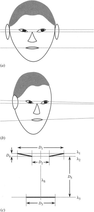
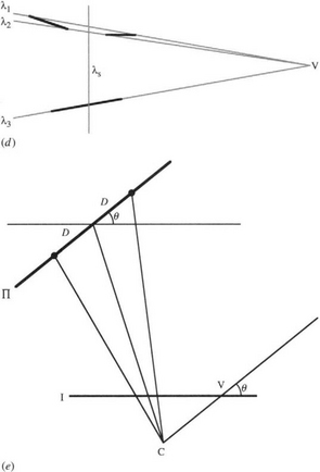
Figure 24.11 3-D analysis of facial parameters. (a) Front view of face. (b) Oblique view of face, showing perspective lines for corners of the eye and mouth. (c) Labeling of eye and mouth features and definition of five interfeature distance parameters. (d) Position of vanishing point under an oblique view. (e) Positions of one pair of features and their midpoint on the facial plane Π. Note how the midpoint is no longer the midpoint in the image plane I when viewed under perspective projection. Note also how the vanishing point V gives the horizontal orientation of Π.

Other facial features, such as the corners of the eye and mouth, can be found by tracking, by snake algorithms, or simply by corner detection. Similarly, the upper and lower contours of the ear and of the nose can be ascertained, thus yielding fixed points that can be used for a multitude of purposes ranging from person identification to recognition of facial expressions. At this point it is useful to reconsider the fact that the face is part of the head and that this is a 3-D object.

24.13 Another Look at Statistical Pattern Recognition: The Support Vector Machine

The support vector machine (SVM) is a new paradigm for statistical pattern recognition and emerged during the 1990s as an important contender for practical applications. The basic concept relates to linearly separable feature spaces and is illustrated in Fig. 24.12a. The idea is to find the pair of parallel hyperplanes that leads to the maximum separation between two classes of feature so as to provide the greatest protection against errors. In Fig. 24.12a, the dashed set of hyperplanes has lower separation and thus represents a less ideal choice, with reduced protection against errors. Each pair of parallel hyperplanes is characterized by specific sets of feature points—the so-called support vectors. In the feature space shown in Fig. 24.12a, the planes are fully defined by three support vectors, though clearly this particular value only applies for 2-D feature spaces. In N dimensions the number of support vectors required is N + 1. This provides an important safeguard against overfitting, since however many data points exist in a feature space, the maximum number of vectors used to describe it is N + 1.

Figure 24.12 Principle of the support vector machine. (a) shows two sets of linearly separable feature points: the two parallel hyperplanes have the maximum possible separation d and should be compared with alternatives such as the pair shown dashed. (b) shows the optimal piecewise linear solution that would be found by the nearest neighbor method.

For comparison, Fig. 24.12b shows the situation that would exist if the nearest neighbor method were employed. In this case the protection against errors would be higher, as each position on the separating surface is optimized to the highest local separation distance. However, this increase in accuracy comes at quite a high cost in the much larger number of defining example patterns. As indicated above, much of the gain of the SVM comes from its use of the smallest possible number of defining example patterns (the support vectors). The disadvantage is that the basic method only works when the dataset is linearly separable.

To overcome this problem, it is possible to transform the training and test data to a feature space of higher dimension where the data do become linearly separable. However, this approach will tend to reduce or even eliminate the main advantage of the SVM and lead to overfitting of the data plus poor generalizing ability. However, if the transformation that is employed is nonlinear, the final (linearly separable) feature space could have a manageable number of dimensions, and the advantage of the SVM may not be eroded. Nevertheless, there comes a point where the basic restriction of linear separability has to be questioned. At that point, it has been found useful to build “slack” variables s_i into the optimization equations to represent the amount by which the separability constraint can be violated. This is engineered by adding a cost term C ∑_i s_i to the normal error function. C is adjustable and acts as a regularizing parameter, which is optimized by monitoring the performance of the classifier on a range of training data.

For further information on this topic, the reader should consult either the original papers by Vapnik, including Vapnik (1998), the specialized text by Cristianini and Shawe-Taylor (2000), or other texts on statistical pattern recognition, such as Webb (2002).

24.14 Concluding Remarks

The methods of this chapter make it rather surprising that so much of image processing and analysis is possible without any reference to a priori probabilities. This situation is likely due to several factors: (1) expediency, and in particular the need for speed of interpretation; (2) the fact that algorithms are designed by humans who have knowledge of the types of input data and thereby incorporate a priori probabilities implicitly, for example, via the application of suitable threshold values; and (3) tacit recognition of the situation outlined in the last section, that probabilistic methods have limited validity and applicability. In practice (following on from the ideas of the last section), it is only at the stage of simple image structure and contextual analysis that probabilistic interpretations come into their own. This explains why SPR is not covered in more depth in this book.

Nonetheless, SPR is extremely valuable within its own range of utility. This includes identifying objects on conveyors and making value judgments of their quality, reading labels and codes, verifying signatures, checking fingerprints, and so on. The number of distinct applications of SPR is impressive, and it forms an essential counterpart to the other methods described in this book.

This chapter has concentrated mainly on the supervised learning approach to SPR. However, unsupervised learning is also vitally important, particularly when training on huge numbers of samples (e.g., in a factory environment) is involved. The section on this topic should therefore not be ignored as a minor and insignificant perturbation. Much the same comments apply to the subject of principal components analysis which has had an increasing following in many areas of machine vision—see Section 24.10. Neither should it go unnoticed that these topics link strongly with those of the following chapter on biologically motivated pattern recognition methods, with artificial neural networks playing a very powerful role.

Section 24.12 is entitled “The Route to Face Recognition” to emphasize that facial analysis involves more than mere statistical pattern recognition. Indeed, this topic is something of a maverick, involving structural pattern recognition and the need to cope with the effects of perspective distortions, variations due to facial plasticity, and the enormous number of individual and interracial variations. A number of these variations can be analyzed with the help of PCA (Gong et al., 2000). As facial analysis is such a wide-ranging topic, we are just considering how some of the crucial features could be identified and related to one another. It is left to the now voluminous literature on the subject to take the discussion further.

24.15 Bibliographical and Historical Notes

Although the subject of statistical pattern recognition does not tend to be at the center of attention in image analysis work,⁷ it provides an important background—especially in the area of automated visual inspection where decisions continually have to be made on the adequacy of products. Most of the relevant work on this topic was already in place by the early 1970s, including the work of Hughes (1968) and Ullmann (1969) relating to the optimum number of features to be used in a classifier. At that stage, a number of important volumes appeared—see, for example, Duda and Hart (1973) and Ullmann (1973) and these were followed a little later by Devijver and Kittler (1982).

The use of SPR for image interpretation dates from the 1950s. For example, in 1959 Bledsoe and Browning developed the n-tuple method of pattern recognition, which turned out (Ullmann, 1973) to be a form of NN classifier. However, it has been useful in leading to a range of simple hardware machines based on RAM (n-tuple) lookups (see for example, Aleksander et al., 1984), thereby demonstrating the importance of marrying algorithms and readily implementable architectures.

Many of the most important developments in this area have probably been those comparing the detailed performance of one classifier with another, particularly with respect to cutting down the amount of storage and computational effort. Papers in these categories include those by Hart (1968) and Devijver and Kittler (1980). Oddly, there appeared to be no overt mention in the literature of how a priori probabilities should be used with the NN algorithm until the author’s paper on this topic (Davies, 1988f): see Section 24.4.

On the unsupervised approach to SPR, Forgy’s (1965) method for clustering data was soon followed by the now famous ISODATA approach of Ball and Hall (1966), and then by MacQueen’s (1967) k-means algorithm. Much related work ensued, which has been summarized by Jain and Dubes (1988), a now classic text. However, cluster analysis is an exacting process, and various workers have felt the need to push the subject further forward. For example, Postaire and Touzani (1989) required more accurate cluster boundaries; Jolion and Rosenfeld (1989) wanted better detection of clusters in noise; Chauduri (1994) needed to cope with time-varying data; and Juan and Vidal (1994) required faster k-means clustering. All this work can be described as conventional and did not involve the use of robust statistics per se. However, elimination of outliers is central to the problem of reliable cluster analysis. For a discussion of this aspect of the problem, see Appendix A and the references listed therein.

Although the field of pattern recognition has moved forward substantially since 1990, fortunately there are several quite recent texts that cover the subject relatively painlessly (Theodoridis and Koutroumbas, 1999; Duda et al., 2001; Webb, 2002). The reader can also appeal to the review article by Jain et al. (2000), which outlines new areas that appeared in the previous decade.

Multiple classifiers is a major new topic and is well reviewed by Duin (2002), a previous review having been carried out by Kittler et al. (1998). Ho et al. (1994) dates from when the topic was rather younger and lists an interesting set of options as seen at that point; some of these are covered in Section 24.8.

Bagging and boosting are further variants on the multiple classifier theme. They were developed by Breiman (1996) and Freund and Schapire (1996). Bagging (short for “bootstrap aggregating”) means sampling the training set, with replacement, n times, generating b bootstrap sets to train b subclassifiers, and assigning any test pattern to the class most often predicted by the subclassifiers. The method is particularly useful for unstable situations (such as when classification trees are used), but is almost valueless when stable classification algorithms are used (such as the nearest neighbor algorithm). Boosting is useful for aiding the performance of weak classifiers. In contrast with bagging, which is a parallel procedure, boosting is a sequential deterministic procedure. It operates by assigning different weights to different training set patterns according to their intrinsic (estimated) accuracy. For further progress with these techniques, see Rätsch et, al. (2002), Fischer and Buhmann (2003), and Lockton and Fitzgibbon (2002). Finally, Beiden et al. (2003) discuss a variety of factors involved in the training and testing of competing classifiers. In addition, much of the discussion relates to multivariate ROC analysis.

Support vector machines (SVMs) also came into prominence during the 1990s and are finding an increasing number of applications. The concept was invented by Vapnik, and the historical perspective is covered in Vapnik (1998). Cristianini and Shawe-Taylor (2000) provide a student-oriented text on the subject.

Progress has also been made in other areas, such as unsupervised learning and cluster analysis (e.g., Mitra et al., 2002; Veenman et al., 2002), but space does not permit further discussion here. Note that, for a more complete view of the modern state of the subject, we must take into account recent work on artificial neural networks (see Chapter 25).

24.16 Problems