Chapter 21. Gas–Liquid Reactions: Penetration Theory Approach

Search in book...
Toggle Font Controls
Create new playlist

Name your new playlist

Playlist description (optional)
Sign In

Email address

Password

Forgot Password?

or

Continue with Facebook

Continue with Google
Sign Up

Full Name

Email address

Confirm Email Address

Password

or

Continue with Facebook

Continue with Google

Chapter 21. Gas–Liquid Reactions: Penetration Theory Approach

Learning Objectives

After completing this chapter, you will be able to:

Model gas absorption with reaction on the basis of the penetration theory.
See the differences between the predictions of the film model and the penetration model.
Understand the use of laboratory-scale contactors with well-established hydrodynamic patterns to find physico-chemical parameters such as rate constant and diffusivity.

Analysis of gas–liquid reactions based on the film model was studied in Chapter 20. An alternative model for mass transfer from a gas–liquid interface is the penetration theory model, which was introduced in Section 8.8. Here we present an analysis of gas–liquid reactions based on the penetration model. It is essentially an exercise in transient diffusion with chemical reaction. Important results and applications result from these models, in particular, in the experimental methods for parameter estimation, and we illustrate these with some examples.

Penetration theory is based on the concept of surface renewal where the surface elements are exposed to gas for a certain time and then replenished by the eddies or flow from the bulk liquid. Thus the concept of stagnant film from the film model is not used and mass transfer from the gas is modeled as a transient process. The enhancement due to reaction can be modeled based on this concept. We illustrate the mathematics to do so, present illustrative results, and show the implications in design and parameter estimation.

The key parameter in the penetration model is the contact time or the exposure time. This is the time for which a gas–liquid interface remains in contact before the eddies sweep the interface and cause mixing at the interface. Laboratory gas–liquid contacters can be designed so that the contact time is precisely known. This permits the determination of other parameters such as diffusion coefficient as well as the rate constant, which can often be difficult to measure, especially for fast reactions. The methodology is illustrated here where we use the penetration theory model as the basis for determination of these parameters.

21.1 Concepts of Penetration Theory

We first briefly review the concepts in penetration theory for mass transfer and follow this with a study of the effect of first-order reactions on the rate of mass transfer based on this theory.

The film model assumes a stagnant film and steady state diffusion with reaction in the film. In actuality the gas–liquid interface is constantly renewed and the steady state profile envisioned in the film model is only an approximation. Nevertheless it has provided a useful tool for correlation of absorption with reaction data and in the design of equipment.

The penetration model is an attempt to improve the situation where we assume a surface element of liquid remains in contact with the gas for a certain time during which a transient diffusion with reaction takes place. A transient concentration profile starts to develop near the interface. After the elapse of a certain amount of time, called the contact time or exposure time, the surface element is assumed to be replaced by an element coming from the bulk element. This sweeps the concentration profile established near the surface and the process starts all over again. See also the discussion in Section 8.8 and the expression for the mass transfer coefficient based on this model for the no-reaction case (Equation 8.49).

21.1.1 First-Order or Pseudo-First-Order Reaction

From the above discussion showing the transient nature of exposure of gas and liquid it is logical to start with the transient diffusion-reaction equation:

\begin{matrix} \frac{\partial C_{A}}{\partial t} = D_{A} \frac{d^{2} C_{A}}{d x^{2}} - k C_{A} & (21.1) \end{matrix}

$\begin{matrix} \frac{\partial C_{A}}{\partial t} = D_{A} \frac{d^{2} C_{A}}{d x^{2}} - k C_{A} & (21.1) \end{matrix}$

Film theory uses a steady state model with a finite film thickness. A semi-infinite region is assumed for the penetration model. The boundary and initial conditions are therefore as follows:

At x = 0, C_A = C*_A, a prescribed interface concentration. This will be equal to the saturation solubility of the gas if there is no gas-side resistance. This is applied for t > 0.
As x → ∞, C_A = C_Ab. Usually the bulk concentration will be zero for reasonably fast irreversible reactions.
The initial condition is C_A = C_Ab for all x for t > 0, the bulk concentration.

The solution is calculated for times 0 to t_E, the exposure time. The instantaneous and average rate of absorption can then be calculated from the concentration gradient at the interface, x = 0:

N_{A 0} (t) = - D_{A} {(\frac{\partial C_{A}}{\partial x})}_{x = 0}

$N_{A 0} (t) = - D_{A} {(\frac{\partial C_{A}}{\partial x})}_{x = 0}$

The average rate is the integral average of this from 0 to t_E:

{\bar{N}}_{A 0} = \frac{1}{t_{E}} \int_{0}^{t_{E}} N (t) d t

${\bar{N}}_{A 0} = \frac{1}{t_{E}} \int_{0}^{t_{E}} N (t) d t$

These are the primary quantities of interest.

The solution to this problem was derived by Danckwerts (1950a) and holds a prominent place in the absorption with chemical reaction literature. Also the books by Astarita (1967) and Danckwerts (1970) are useful resources for a detailed study of gas–liquid reactions. The Laplace transform is useful for such problems and we will study the use of this method here.

21.1.2 Laplace Transform Method

We define ${\bar{C}}_{A}$ ${\bar{C}}_{A}$ as the Laplace transform, which is a function of the transform variable s:

{\bar{C}}_{A} = \int_{0}^{\infty} C_{A} (t) \exp (- s t) d t

${\bar{C}}_{A} = \int_{0}^{\infty} C_{A} (t) \exp (- s t) d t$

This reduces the PDE in Equation 21.1 to an ODE:

\begin{matrix} D_{A} \frac{d^{2} {\bar{C}}_{A}}{d x^{2}} - (s + k) {\bar{C}}_{A} = 0 & (21.2) \end{matrix}

$\begin{matrix} D_{A} \frac{d^{2} {\bar{C}}_{A}}{d x^{2}} - (s + k) {\bar{C}}_{A} = 0 & (21.2) \end{matrix}$

where we have used an initial condition of zero, that is, C_Ab = 0, which is valid for fast reactions.

The boundary condition at the surface in the Laplace domain is C*_A/s, which holds for x = 0. (Note that this is for a step change in the concentration at the surface, the problem being studied here.) Hence the solution to Equation 21.2 is

\begin{matrix} {\bar{C}}_{A} (x, s) = (\frac{C_{A}^{*}}{s}) \exp (- x \sqrt{\frac{s + k}{D_{A}}}) & (21.3) \end{matrix}

$\begin{matrix} {\bar{C}}_{A} (x, s) = (\frac{C_{A}^{*}}{s}) \exp (- x \sqrt{\frac{s + k}{D_{A}}}) & (21.3) \end{matrix}$

Students should verify the algebra leading to this equation at this stage. All that remains is to find the inverse transform to find the solution in the time domain. Easier said than done! Tables of inverse transforms are available for a large class of problems including this one and can be directly used. Computer algebra based on MAPLE or MATHEMATICA can also be used. We will skip the mathematics and present the final solution in the time domain:

\begin{matrix} \begin{array}{r} \frac{C_{A} (x, t)}{C_{A}^{*}} = \frac{1}{2} \exp (- x \sqrt{k / D_{A}}) erfc (\frac{x}{2 \sqrt{D_{A} t}} - \sqrt{k t}) \\ + \frac{1}{2} \exp (x \sqrt{k / D_{A}}) erfc (\frac{x}{2 \sqrt{D_{A} t}} + \sqrt{k t}) \end{array} & (21.4) \end{matrix}

$\begin{matrix} \begin{array}{r} \frac{C_{A} (x, t)}{C_{A}^{*}} = \frac{1}{2} \exp (- x \sqrt{k / D_{A}}) erfc (\frac{x}{2 \sqrt{D_{A} t}} - \sqrt{k t}) \\ + \frac{1}{2} \exp (x \sqrt{k / D_{A}}) erfc (\frac{x}{2 \sqrt{D_{A} t}} + \sqrt{k t}) \end{array} & (21.4) \end{matrix}$

The profiles with and without reaction are illustrated in Figure 21.1 for two values of the rate constant for a fixed value of time equal to 1 sec.

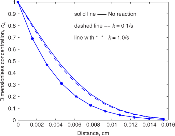
A line graph to plot the dimensionless concentration versus distance.

Figure 21.1 Illustrative concentration profiles for transient diffusion with reaction in a semi-infinite region; the slow reaction case shows little difference between the reacting and non-reacting cases. D_A = 2 × 10^–5 cm²/s and t = 1 sec for the calculations.

The interesting behavior is that there is not much difference between physical and chemical absorption for small values of the rate constant (k = 0.1 s^–1 in the figure). Hence we will not expect much enhancement in the rate due to reaction. This is similar to the slow reaction case anticipated by the film model.

For a rate constant of k = 1 s^–1 we see that the profiles are different for the reaction (marked with *) and no-reaction cases (solid line). In particular the absolute value of the slope of the profile at the interface is larger, showing that the reaction enhances the rate of mass transfer.

Figure 21.2 shows the effect of a larger value of the rate constant, k = 10 s^–1, for two values of time. The concentration front for the reaction case hardly moves inward toward the liquid bulk and appears to be stagnated in contrast to the no-reaction case. Here the profiles for a reaction are close to a steady state solution and are represented as

\begin{matrix} \frac{C_{A} (x, t)}{C_{A}^{*}} = \exp (- x \sqrt{k / D_{A}}) & (21.5) \end{matrix}

$\begin{matrix} \frac{C_{A} (x, t)}{C_{A}^{*}} = \exp (- x \sqrt{k / D_{A}}) & (21.5) \end{matrix}$

A line graph to plot the concentration versus distance.

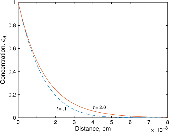
Figure 21.2 Illustrative concentration profiles for transient diffusion with reaction in a semi-infinite region for a fast reaction: k = 10/s; D_A = 2 × 10^–5 cm²/s. Solutions are presented for t = 0.1 sec and t = 2 sec and show that the rate movement of the concentration front is rather small. Diffusion balances reaction here and a nearly steady state profile is reached quickly.

In this case the effect of contact time will not be to be of importance and the concentration profile is established mainly by a balance of diffusion and reaction at each spatial location. The steady state–based film model would have given the same prediction. The value of the mass transfer coefficient is not important here, similar to the pseudo-first-order case in the film model. These differences are important in analyzing experimental data based on the penetration theory as discussed later. Thus by changing the contact time or time of exposure of the system, we can determine both the diffusion coefficient and the rate constant depending on the parameter that has the most dominant effect on the rate of absorption.

The key conclusions are that at low contact times, reaction does not enhance the rate of mass transfer, while at large contact times, the reaction is balanced by diffusion and the contact time does not play a significant role. The characteristic dimensionless parameter is kt_E in the penetration model. The effect of this parameter on the flux is shown next.

21.1.3 Flux and the Average Rate of Mass Transfer

The flux of A at the surface in the presence of reaction is of more practical importance and can be calculated from the following formula derived from Equation 21.4 by applying Fick’s law at the interface:

\begin{matrix} N_{A 0} (t) = C_{A}^{*} \sqrt{D_{A} k} [erf (\sqrt{k t}) + \frac{\exp (- k t)}{\sqrt{(π k t)}}] & (21.6) \end{matrix}

$\begin{matrix} N_{A 0} (t) = C_{A}^{*} \sqrt{D_{A} k} [erf (\sqrt{k t}) + \frac{\exp (- k t)}{\sqrt{(π k t)}}] & (21.6) \end{matrix}$

This is the instantaneous flux and it decreases with increase in time.

The more useful result is the average flux over a time interval t_E. This is calculated as an integral of the instantaneous flux with respect to time and then dividing by t_E. The result is

\begin{matrix} {\bar{N}}_{A 0} = C_{A}^{*} \sqrt{\frac{D_{A}}{k t_{E}^{2}}} [(k t_{E} + 1 / 2) erf (\sqrt{k t_{E}}) + \exp (- k t_{E}) \sqrt{\frac{k t_{E}}{π}}] & (21.7) \end{matrix}

$\begin{matrix} {\bar{N}}_{A 0} = C_{A}^{*} \sqrt{\frac{D_{A}}{k t_{E}^{2}}} [(k t_{E} + 1 / 2) erf (\sqrt{k t_{E}}) + \exp (- k t_{E}) \sqrt{\frac{k t_{E}}{π}}] & (21.7) \end{matrix}$

This provides the rate of absorption based on the penetration theory for reaction with a first order-reaction.

The enhancement factor is obtained by dividing by the no reaction value given by Equation 8.43, which is repeated here for ease of reference:

{\bar{N}}_{A 0} no reaction = = (2 \sqrt{\frac{D_{A}}{π t_{E}}}) C_{A}^{*}

${\bar{N}}_{A 0} no reaction = = (2 \sqrt{\frac{D_{A}}{π t_{E}}}) C_{A}^{*}$

The bracketed quantity on the right-hand side is the value of the mass transfer coefficient according to the penetration theory. Hence the enhancement factor for a first-order (or pseudo-first-order) reaction according to the penetration model is

\begin{matrix} \begin{matrix} E = \frac{\sqrt{π}}{2 \sqrt{k t_{E}}} [(k t_{E} + 1 / 2) erf (\sqrt{k t_{E}}) + \exp (- k t_{E}) \sqrt{\frac{k t_{E}}{π}}] \end{matrix} & (21.8) \end{matrix}

$\begin{matrix} \begin{matrix} E = \frac{\sqrt{π}}{2 \sqrt{k t_{E}}} [(k t_{E} + 1 / 2) erf (\sqrt{k t_{E}}) + \exp (- k t_{E}) \sqrt{\frac{k t_{E}}{π}}] \end{matrix} & (21.8) \end{matrix}$

Note that the dimensionless parameter kt_E plays the role of the Hatta number in the penetration model. Hatta is not used here unlike the film model since there is no well-defined film thickness because we deal with a semi-infinite region in the penetration model. The two models will be compared next.

21.1.4 Relation between Film Theory and Penetration Theory

If k_L from penetration theory is used in the definition of the Hatta number the following relation is obtained:

\begin{matrix} H a^{2} = \frac{π}{4} (k t_{E}) & (21.9) \end{matrix}

$\begin{matrix} H a^{2} = \frac{π}{4} (k t_{E}) & (21.9) \end{matrix}$

This can be used to connect the two models for reacting systems.

The enhancement factor when Ha is small based on the film theory can be approximated as

E = 1 + \frac{H a^{2}}{3} for H a \approx < 1

$E = 1 + \frac{H a^{2}}{3} for H a \approx < 1$

This is close to that predicted by the penetration theory, which gives the following value (see exercise problem 21.2):

E = \frac{1}{2} (1 + k t) for k t_{E} \approx < 1

$E = \frac{1}{2} (1 + k t) for k t_{E} \approx < 1$

The differences between the film and penetration models become even smaller for larger Ha. The enhancement factor based on the film theory is equal to Ha for Ha > 3. For this case penetration theory also predicts the same value if a Hatta number is defined as per Equation 21.9. Overall the two approaches lead to very similar results and the model choice is merely a matter of preference for reacting systems.

21.2 Bimolecular Reaction

Now we consider a case where rate depends on the concentration of both A and B. Species A (dissolved gas) diffuses from the interface to the bulk while species B (the liquid phase reactant) counter-diffuses toward the interface. Hence the model is set up by using the transient diffusion equation for both species A and B.

The rate term in Equation 21.1 is now modified with a second-order term and the differential equation for A is

\begin{matrix} \frac{\partial C_{A}}{\partial t} = D_{A} \frac{d^{2} C_{A}}{d x^{2}} - k_{2} C_{A} C_{B} & (21.10) \end{matrix}

$\begin{matrix} \frac{\partial C_{A}}{\partial t} = D_{A} \frac{d^{2} C_{A}}{d x^{2}} - k_{2} C_{A} C_{B} & (21.10) \end{matrix}$

An additional equation for B is used in conjunction with this:

\begin{matrix} \frac{\partial C_{B}}{\partial t} = D_{B} \frac{d^{2} C_{B}}{d x^{2}} - ν k_{2} C_{A} C_{B} & (21.11) \end{matrix}

$\begin{matrix} \frac{\partial C_{B}}{\partial t} = D_{B} \frac{d^{2} C_{B}}{d x^{2}} - ν k_{2} C_{A} C_{B} & (21.11) \end{matrix}$

A numerical solution is needed but gets more involved due to a sharp-moving type of front near the interface. The equations are solved using dimensionless variables. Let us see what dimensionless variables should be used.

21.2.1 Dimensionless Form of the Model

Scaling of the concentration is the same as before in the film theory with c_A and c_B defined as dimensionless concentrations. Since the solution is sought for time up to t_E this can be used as the reference time scale. Hence τ = t/t_E. The distance is now scaled with $\sqrt{D_{A} t_{E}}$ $\sqrt{D_{A} t_{E}}$ . Hence $Ξ = x / \sqrt{D_{A} t_{E}}$ $Ξ = x / \sqrt{D_{A} t_{E}}$ is defined as the dimensionless distance. The dimensionless representation is therefore

\begin{matrix} \frac{\partial c_{A}}{\partial τ} = \frac{d^{2} c_{A}}{d ξ^{2}} - M c_{A} c_{B} & (21.12) \end{matrix}

$\begin{matrix} \frac{\partial c_{A}}{\partial τ} = \frac{d^{2} c_{A}}{d ξ^{2}} - M c_{A} c_{B} & (21.12) \end{matrix}$

where M is defined as

\begin{matrix} M = k_{2} C_{B L} t_{E} & (21.13) \end{matrix}

$\begin{matrix} M = k_{2} C_{B L} t_{E} & (21.13) \end{matrix}$

This plays a role similar to the Hatta number.

An additional equation for B is used in conjunction with Equation 21.12:

\begin{matrix} \frac{\partial c_{B}}{\partial τ} = \frac{D_{B}}{D_{A}} \frac{d^{2} c_{B}}{d ξ^{2}} - \frac{M c_{A} c_{B}}{q} & (21.14) \end{matrix}

$\begin{matrix} \frac{\partial c_{B}}{\partial τ} = \frac{D_{B}}{D_{A}} \frac{d^{2} c_{B}}{d ξ^{2}} - \frac{M c_{A} c_{B}}{q} & (21.14) \end{matrix}$

Here q is the additional dimensionless group needed and is defined as the concentration ratio parameter:

\begin{matrix} q = \frac{C_{B L}}{ν C_{A}^{*}} & (21.15) \end{matrix}

$\begin{matrix} q = \frac{C_{B L}}{ν C_{A}^{*}} & (21.15) \end{matrix}$

Note that this does not include the diffusivity ratio D_B/D_A (unlike the film model). The diffusivity ratio appears as a separate parameter. Hence three dimensionless quantities are involved. The film model needs only two since the diffusivity ratio does not appear as an independent parameter.

The quantity of interest is ${\bar{N}}_{A 0}$ ${\bar{N}}_{A 0}$ , the time-averaged value of flux over a period of t_E. The results are expressed in terms of an enhancement factor:

E = \frac{{\bar{N}}_{A 0}}{2 C_{A}^{*}} \sqrt{\frac{π t_{E}}{D_{A}}}

$E = \frac{{\bar{N}}_{A 0}}{2 C_{A}^{*}} \sqrt{\frac{π t_{E}}{D_{A}}}$

21.2.2 Illustrative Results

An illustrative solution for the concentration profiles of A and B is presented in Figure 21.3, which illustrates how the profiles evolve with time.

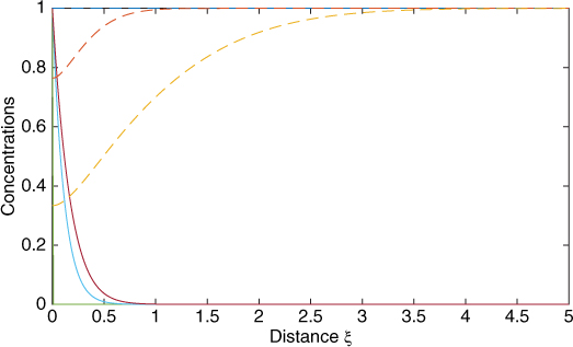
Figure 21.3 Evolution of the concentration profiles for A (solid lines) and B (dotted lines) with time for a second-order (1,1) reaction simulated by the PDEPE solver. M = 10 and q = 10. Profiles shown for dimensionless times τ = 0.1 and 10.

Numerical solutions for this figure were generated using the PDEPE solver introduced in Section 8.11. Due to steep profiles near the interface a large number of mesh points in space is needed. Further, the semi-infinite space domain needs to truncated with a finite domain (usually an ξ of 5 is adequate). Also, to find the average flux and the enhancement factor, sufficient evaluation points in time are also needed so that the time integration is also accurate. The enhancement factor for the data used in Figure 20.3 was computed as 7.25 using numerical flux values calculated at equal-spaced times and then using the trapezoidal rule. This is close to the film model solution value of 7.07.

21.3 Instantaneous Reaction Case

A special case of the bimolecular reaction is reached for large values of M (at a fixed q value) and the instantaneous reaction asymptote is reached. This is similar to the film model analyzed in Section 20.3.2 where the instantaneous reaction asymptote is reached for large values of the Hatta number. Illustrative concentration profiles are shown in Figure 21.4 when the reaction is instantaneous.

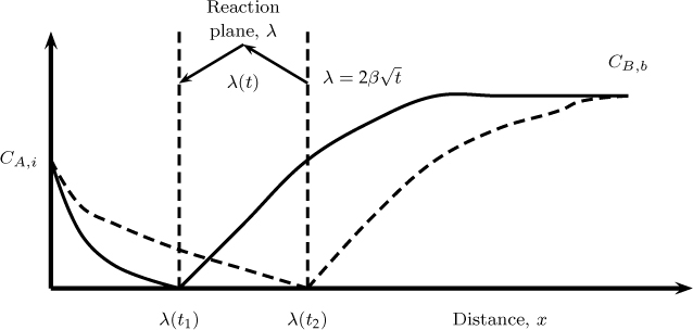
A graph showing the concentration profiles for instantaneous reaction cases.

Figure 21.4 Concentration profiles for A and B for an instantaneous reaction based on the penetration model for mass transfer. Solid lines represent the profiles line at time t₁ and the dashed lines at a larger time t₂.

The reaction front is assumed to be of thickness λ, similar to the film model. Thus we have a no B zone from 0 to λ and a no A zone from λ onwards, similar to the film theory. The main difference here is that the front moves with time inward. The second difference is that a semi-infinite domain is assumed and the domain of the solution for B is not fixed.

The expression for the front movement can be derived by a mass balance at the interface. The solution was derived by Danckwerts (1951). The reaction front separates species A and B. Only A is present in the region 0 to λ. Transient diffusion with no reaction applies here. It can be shown that the following equation satisfies both the differential condition and the boundary condition at x = 0:

\begin{matrix} c A = 1 - A_{2} erf (x / 2 \sqrt{D_{A} t}) & (21.16) \end{matrix}

$\begin{matrix} c A = 1 - A_{2} erf (x / 2 \sqrt{D_{A} t}) & (21.16) \end{matrix}$

Here A₂ is an integration constant. Now using the boundary condition that c_A = 0 at x = λ we can evaluate the integration constant:

\begin{matrix} A_{2} = \frac{1}{erf (λ / 2 \sqrt{D_{A} t})} & (21.17) \end{matrix}

$\begin{matrix} A_{2} = \frac{1}{erf (λ / 2 \sqrt{D_{A} t})} & (21.17) \end{matrix}$

If A₂ has to remain constant and should not vary with time, then λ must be proportional to the square root of time and we can suggest that the following relation should hold for the front movement:

\begin{matrix} λ = 2 β \sqrt{t} & (21.18) \end{matrix}

$\begin{matrix} λ = 2 β \sqrt{t} & (21.18) \end{matrix}$

Here β is a constant to be determined.

A similar analysis for the B-rich zone gives the following equation for the concentration profile of B:

\begin{matrix} c_{B} = \frac{erfc (x / 2 \sqrt{D_{A} t}) - erf (β / \sqrt{t})}{erfc (β / \sqrt{t})} & (21.19) \end{matrix}

$\begin{matrix} c_{B} = \frac{erfc (x / 2 \sqrt{D_{A} t}) - erf (β / \sqrt{t})}{erfc (β / \sqrt{t})} & (21.19) \end{matrix}$

The fluxes at λ from both sides should match and this can be now used to find β. The following implicit expression is obtained after some algebra:

\begin{matrix} \exp (β^{2} / D_{B}) erfc (β / \sqrt{D_{B}}) = \frac{C_{B L}}{ν C_{A}^{*}} \sqrt{\frac{D_{B}}{D_{A}}} \exp (β^{2} / D_{A}) erf (β / \sqrt{D_{A}}) & (21.20) \end{matrix}

$\begin{matrix} \exp (β^{2} / D_{B}) erfc (β / \sqrt{D_{B}}) = \frac{C_{B L}}{ν C_{A}^{*}} \sqrt{\frac{D_{B}}{D_{A}}} \exp (β^{2} / D_{A}) erf (β / \sqrt{D_{A}}) & (21.20) \end{matrix}$

The flux of A at the interface can now be calculated by applying Fick’s law and the result is

\begin{matrix} N_{A 0} (t) = \frac{C_{A *}}{erf (β / \sqrt{D_{A}})} \sqrt{\frac{D_{A}}{π t}} & (21.22) \end{matrix}

$\begin{matrix} N_{A 0} (t) = \frac{C_{A *}}{erf (β / \sqrt{D_{A}})} \sqrt{\frac{D_{A}}{π t}} & (21.22) \end{matrix}$

Simplified results apply when E >> 1. In such case we have

E = \sqrt{\frac{D_{A}}{D_{B}}} + \frac{C_{B L}}{ν C_{A}^{*}} \sqrt{\frac{D_{B}}{D_{A}}}

$E = \sqrt{\frac{D_{A}}{D_{B}}} + \frac{C_{B L}}{ν C_{A}^{*}} \sqrt{\frac{D_{B}}{D_{A}}}$

It can be shown that the enhancement factor predicted by the film and penetration models are identical if D_A = D_B. A somewhat approximate but useful generalization follows if the film theory parameter q is corrected as follows: the film theory parameter q defined as (D_B/D_A)(C_BL/νC*_A) is modified by taking the square root of diffusivity and is defined as

q = \frac{C_{B L}}{ν C_{A}^{*}} \sqrt{\frac{D_{B}}{D_{A}}}

$q = \frac{C_{B L}}{ν C_{A}^{*}} \sqrt{\frac{D_{B}}{D_{A}}}$

If the expression E = 1 + q in the film theory model is used with this modified q, then the film model solution is nearly the same as the penetration model. This is known as the square root diffusivity correction of the film model. An application of the model is illustrated in Example 21.1

Example 21.1 H₂S Absorption in an Amine Solution

H₂S is absorbed in a 0.1 M solution of the amine, MEA, at 25°C and the reaction can be taken as instantaneous and irreversible. The solubility coefficient of H₂S is 0.1 mol/L atm, the diffusion coefficient is 1.48 × 10^–5 cm²/s and D_B/D_A = 0.64. The gas and liquid are in contact for a time of 0.1 seconds. Find up to what point the reaction front has moved, the value of the enhancement factor and the rate of absorption. Compare with the value obtained from the film model.

Solution

Equation 21.20 is solved in MATLAB using the function FZERO. It is easier to solve in terms of $β / \sqrt{D_{A}}$ $β / \sqrt{D_{A}}$ as a parameter. The value is found as 0.511 and hence β = 0.002. The reaction front therefore moves with the square root of time with a proportionality constant of 2β. If the liquid is exposed for 0.1 seconds, a B-depleted layer of 0.02 cm will develop near the surface.

The enhancement factor is calculated using Equation 21.22 as 1.8859.

The film theory model will predict with a corrected value of q an enhancement factor of 1.64.

The rate of absorption is calculated as k_L C*_AE.

The k_L in turn is calculated from the penetration model as 2 (D/πt_E)^0.5.

The results for a H₂S partial pressure of 1 atm are as follows:

k_L = 1.84 × 10^–4cm/s and N_A = 3.25 × 10^–8mol/cm² s.

Having discussed the penetration model in some detail, we next discuss ideal contactors for measurement of experimental data in gas–liquid reacting systems.

21.4 Ideal Contactors

Ideal contactors refer to gas–liquid absorption equipment where the hydrodynamics is known and the time of exposure can be calculated independently. This permits the evaluation of diffusion and reaction rate constants. We present some of the commonly used ideal contactors and illustrate how they are useful for parameter evaluation.

In general they can be classified into two broad categories (adapted from Mills et al., 1992):

Category A: Both the hydrodynamics and interfacial area are theoretically known. Examples are the laminar jet apparatus and wetted wall and wetted sphere columns discussed in this section.
Category B: Only the interfacial area is known but the mass transfer coefficient is not well characterized. An example is the stirred cell.

A brief description of these categories of contactors is provided in the following section.

21.4.1 Laminar Jet Apparatus

In this device, a jet of liquid enters a gas space through a circular hole and leaves out a slightly larger hole. The time of exposure of the liquid is calculated by assuming the jet is a cylindrical rod with a uniform velocity, υ:

t_{E} = \frac{L}{v} = \frac{π d^{2} L}{4 Q}

$t_{E} = \frac{L}{v} = \frac{π d^{2} L}{4 Q}$

Here L is the length of the jet, d its diameter, and Q the volumetric liquid flow rate. The time of exposure can be varied by changing L or Q or both. A modified design where the gas is mildly agitated without disturbing the flow in the jet is presented in Figure 21.5.

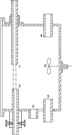
A diagram of the wetted wall column is shown. The parts are numbered from 1 to 6.

Figure 21.5 Sketch of the laminar jet apparatus. A modified design from Bjerle (1972) is shown where the gas is mixed with mild agitation using a propeller (6). This reduces the gas-side resistance. 1. Transmission nozzle; 2. receiver nozzle; 3. gas inlet; 4. gas outlet; 5. drain.

The mild agitation of the gas reduces the gas-side resistance and makes the data interpretation less sensitive to the value of the gas-side mass transfer coefficient. Note that if pure gas is used then the gas-side resistance is nonexistent but this may not be always feasible to do so due to other considerations, for example, temperature rise due to heat of the solution and absorption.

21.4.2 Wetted Wall Column

In the wetted wall column, the liquid flows down as a film under the influence of gravity over a surface, usually a rod or a tube. A number of design variations have been used in the literature. One design of Roberts and Danckwerts (1962) is shown in Figure 21.6.

A diagrammatical representation of a wetted wall column is shown.

Figure 21.6 Sketch of a wetted wall column.

The mass transfer coefficient can be predicted by the contact time at the interface. This in turn is equal to the length of the tube over which the liquid is flowing and the velocity at the surface. The liquid velocity at the surface is υ_max for the falling film given in Section 10.5.2. This depends on the film thickness, which in turn depends on the liquid flow rate. Combining all these, the following expression is obtained for the velocity at the surface:

v_{s} = \frac{3}{2} {(\frac{Q}{π d})}^{2 / 3} {(\frac{ρ g}{3 μ})}^{1 / 3}

$v_{s} = \frac{3}{2} {(\frac{Q}{π d})}^{2 / 3} {(\frac{ρ g}{3 μ})}^{1 / 3}$

where d is the diameter of the tube over which the liquid flows. The expression assumes that the film flow is in the laminar regime.

The contact time is therefore equal to L/υ_s. The interfacial area is equal to the geometric area of the gas–liquid interface in the absence of waves or ripples. This is equal to πdL.

The range of k_L values is 2 × 10^–5m/s to 2 × 10^–4m/s, comparable to that in a stirred cell. The area to volume parameter is small and on the order of 2 × 10^–2 m^–1 Hence it can be used as a model for simulation of packed columns since the coefficient values in a packed column are in a similar range.

21.4.3 Wetted Sphere

A contactor similar in concept is the wetted sphere column, shown in Figure 21.7.

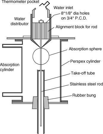
A diagrammatical representation of a wetted sphere is shown.

Figure 21.7 Sketch of a wetted sphere apparatus.

Here the liquid flows over a spherical surface rather than on a rod. The advantage over the wetted wall column is that ripples as well as the end effects are reduced. The disadvantage is that data interpretation is complicated due to the converging-diverging flow over the sphere. A detailed solution to the velocity profile was presented by Davidson and Cullen (1957) and this work can be used to find the contact time. Mashelkar and Soylu (1974) used this to measure the diffusion coefficient of solutes for several non-Newtonian and viscoelastic solvents.

21.4.4 Stirred Cells

In this contactor, shown in Figure 21.8 (a design due to Levenspiel and Godfrey, 1974), the gas and liquid are separated by an interface of known area.

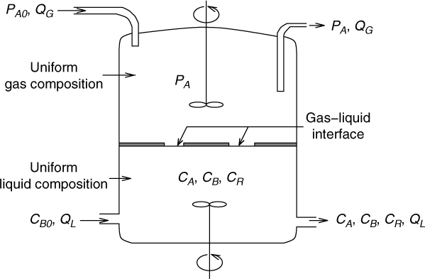
A schematic diagram of a stirred cell is shown.

Figure 21.8 Sketch of a stirred cell. The modified design by Levenspiel and Godfrey (1974) is illustrated here.

In this design there are two flanged sections, the upper section for the gas and the lower for the liquid. Both sections are mildly agitated with the stirrers provided for each section. A plate with holes separates the two sections. The interfacial area can be varied by using plates with varying numbers of holes with varying diameters and is therefore known precisely.

The mass transfer coefficient is not known and has to be determined separately by independent experiments. The k_L values are seen to be in the range of 2 × 10^–5 m/s to 2 × 10^–4 m/s, which is comparable to a wetted wall column. The area to volume parameter is small and on the order of 2 × 10^–2 m^–1.

If the reaction is in pseudo-first-order conditions this can be verified easily since the rate is then proportional only to the interfacial area, which is known. The parameter $\sqrt{D_{A} k_{1}}$ $\sqrt{D_{A} k_{1}}$ is then obtained directly using the experimental rate of absorption. The rate constant in turn can be found if the diffusion coefficient is either known or independently measured.

Summary

Penetration theory is an attempt to improve the film model by assuming a transient concentration profile near the gas–liquid interface rather than a steady state profile.
The key parameter is the exposure time or contact time. The mass transfer coefficient in a non-reacting system can be directly predicted if the exposure time is known.
For reacting systems a transient diffusion with reaction problem is solved to find the concentration profiles near the interface and the corresponding values of the time-dependent flux.
The time-dependent flux is integrated with respect to time and averaged over the exposure time to get the value of the (averaged) rate of absorption. This is the penetration model for gas–liquid reacting systems.
An analytical solution (lengthy) can be derived for first-order or pseudo-first-order reactions. The average rate is divided by the rate for the no-reaction case to get Equation 21.8 for the enhancement factor.
For a bimolecular reaction, species A and B counter-diffuse toward each other. The transient diffusion with reaction is solved for both species. A solver such as PDEPE is useful although it may be noted that the concentration gradients near the interface are rather sharp and hence a large number of mesh points may be needed near the interface. Other “tailor made” methods may be preferable.
If the bimolecular reaction can be treated as instantaneous, a simpler approach can be used. A reaction front is postulated and this moves inward as a function of time. The location and the movement of the front can be calculated analytically and the enhancement factor can be predicted without a numerical solution.
Penetration theory predictions are often close to film theory unless the diffusivity ratio of A to B is large. Therefore film theory is often still used after replacing the diffusivity ratio in the q parameter by its square root. The simpler film model then gives results close to penetration theory.
Experimental values of rate constants are difficult to measure, especially if the diffusional effects interfere. Hence contactors with known values of mass transfer coefficient and/or interfacial area are to be preferred for laboratory studies. These are referred to as “ideal” gas–liquid reactors and some designs of these contactors are provided in the chapter.
Penetration theory analysis of gas–liquid reactions is an elegant application of the transient diffusion-reaction model and is well worth the study even if you are not going to deal with gas–liquid reactions in your work or prefer to use the film model as an alternative.

Review Questions

21.1 What is meant by exposure time or contact time?

21.2 Does mass transfer coefficient increase or decrease with exposure time?

21.3 What is the dependency of the mass transfer coefficient on the diffusion coefficient when working with the penetration model?

21.4 What form does Equation 21.4 reduce to for k → 0?

21.5 What is the key dimensionless parameter in the penetration model for a first-order reaction? How is the Hatta number related to this parameter?

21.6 What is the difference in enhancement factor for the film and penetration models for Ha = 3? Assume a pseudo-first-order reaction.

21.7 What are the key dimensionless parameters in the penetration model for a bimolecular (second-order) reaction with a moderate depletion of B near the interface?

21.8 What are the key dimensionless parameters in the penetration model for an instantaneous reaction?

21.9 How does the location of the reaction plane change with time for an instantaneous reaction?

21.10 State the use of the square root diffusivity correction for the film model.

21.11 What is meant by an ideal gas–liquid contactor?

21.12 What is the range of k_L values that can be expected in a wetted wall column, strirred cell, and jet apparatus?

Problems

21.1 Verification of the penetration theory solution. Verify that Equation 21.4 satisfies the required boundary conditions as a well as the initial conditions. MAPLE or MATHEMATICA may turn out to be helpful.

21.2 Instantaneous flux directly from Laplace solution. From the Laplace solution given by Equation 21.3 show that the instantaneous flux in the Laplace domain is

{\bar{N}}_{A 0} (s) = (\frac{C_{A}^{*}}{s}) \sqrt{D_{A} s + k}

${\bar{N}}_{A 0} (s) = (\frac{C_{A}^{*}}{s}) \sqrt{D_{A} s + k}$

Look up a table of inverse transforms or invert it using MATHEMATICA or similar tools to verify the expression for the instantaneous flux in the time domain given by Equation 21.6.

21.3 Limiting value of the fluxes for low kt. Show that the flux expression in Equation 21.7 for the rate gas absorption can be simplified for small values of kt as

{\bar{N}}_{A 0} = C_{A}^{*} \sqrt{\frac{D_{A}}{π t}} (1 + k t) for k t < < 1

${\bar{N}}_{A 0} = C_{A}^{*} \sqrt{\frac{D_{A}}{π t}} (1 + k t) for k t < < 1$

Show that the solution error is on the order of 5% for kt = 0.5. Find the total quantity of gas absorbed to t_E for this case. Find the average rate of absorption. If the average rate is divided by k_LC*_A we can obtain an expression for the enhancement factor. Here k_L can be calculated using the penetration model.

21.4 Limiting value of the fluxes for large kt. Show that the flux expression in Equation 21.7 for gas absorption can be simplified for large values of kt and the result is

{\bar{N}}_{A 0} = C_{A}^{*} \sqrt{D_{A} k} for k t > > 1

${\bar{N}}_{A 0} = C_{A}^{*} \sqrt{D_{A} k} for k t > > 1$

Show that the solution error is on the order of 3% for kt = 2.0. Find the total quantity of gas absorbed from time 0 to t_E for this case. Find the average rate of absorption. Compare with the film model. State why there is no difference between the penetration model and the film model.

21.5 Use of penetration model in finding the rate constant. A gas stream with CO₂ at 1 atm partial pressure is exposed to a liquid in which it undergoes a first-order reaction for a time of 0.01 s. The total amount of gas absorbed during this time was measured as 1.5 × 10^–4 moles/m². Estimate the rate constant for this reaction. Use C*_A = 30 mol/m³ and D_A = 1.5 × 10^–9 m²/s.

21.6 Bimolecular reaction: numerical solution. Examine the effect of time of exposure on the rate of absorption of CO₂ in ammonia solution for the following set of parameters. Find the enhancement factor for these values of time. The reaction is second order with a rate constant of 30 L/mol.s. The reaction is assumed irreversible and the dissolved concentration of CO₂ in the bulk liquid is zero. The diffusion coefficients are D_A = D_B = 2 × 10^–5 cm²/s. The saturation solubility for the given condition is 4 × 10^–5 mol/m³ and the ammonia concentration in the bulk is 1 M.

21.7 Instantaneous reaction: analytic solution for reaction front. State the differential equation and the boundary conditions for the A-rich zone and verify that Equation 21.16 holds for the concentration of A in this zone. Similarly verify that Equation 21.19 for B satifies the governing differential equation and the boundary condition. State the matching condition for the fluxes at λ from both sides and use this to derive the expression for β given in the text. Show that the flux of A at the interface is given by

N_{A 0} (t) = \frac{C_{A}^{*}}{erf (β / \sqrt{D_{A}})} \sqrt{\frac{D_{A}}{π t}}

$N_{A 0} (t) = \frac{C_{A}^{*}}{erf (β / \sqrt{D_{A}})} \sqrt{\frac{D_{A}}{π t}}$

Finally, find the average flux and confirm that the enhancement factor is given by Equation 21.22 in the text.

21.8 Penetration theory analysis for absorption of two gases. Simultaneous absorption of two gases with a common reacting liquid phase species was studied by Goettler and Pigford (1971) based on the penetration theory. Set up the model for this, identify the dimensionless parameters, and set up a computational module in MATLAB. Also calculate the enhancement factor for each gas and the ratio of absorption rate of A relative to B for selected values of the dimensionlesss groups.

21.9 Penetration model for two gases, both reacting instantaneously. Extend the penetration model for two species reacting instantaneously. The anticipated concentration profile is shown in Figure 21.9.

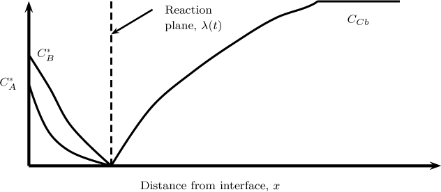
A graph shows the concentration profiles for two gases.

Figure 21.9 Concentration profiles for two gases both reacting instantaneously with a common liquid phase reactant B.

Assume the solution on either side of the interface can be expressed in terms of an error function that obviously satisfies the differential equation. Fit the boundary conditions for each side of the interface. Now use the flux balance at the reaction plane and derive an expression for λ as a function of time. How does this model compare with the film model? Compare the results with the work of Goettler and Pigford (1971).

21.10 Danckwerts surface renewal model. Danckwerts modified the Higibe model by suggesting that there is a distribution of surface ages rather than a single age equal to the contact time. He proposed that the chance of a surface element being replaced is independent of the time for which it has been exposed. Based on this hypothesis the fraction of the surface that has been exposed for time t and t + dt can be shown to equal s exp(–st), where s is the fraction of the surface replaced with fresh liquid in unit time. Verify the following integrals, which are the zeroth and first moment of the surface age distribution function:

\begin{array}{l} μ_{0} = \int_{0}^{\infty} s \exp (- s t) = 1 \\ μ_{1} = \int_{0}^{\infty} t s \exp (- s t) = \frac{1}{s} \end{array}

$\begin{array}{l} μ_{0} = \int_{0}^{\infty} s \exp (- s t) = 1 \\ μ_{1} = \int_{0}^{\infty} t s \exp (- s t) = \frac{1}{s} \end{array}$

This parameter s is therefore representative of the frequency of surface renewal or the reciprocal of the average age of a surface. Derive the following expression for the instantaneous rate of absorption:

{\bar{N}}_{A 0} = \int_{0}^{\infty} s \exp (- s t) N (t) d t

${\bar{N}}_{A 0} = \int_{0}^{\infty} s \exp (- s t) N (t) d t$

Show that the use of these relations leads to the following expression for the mass transfer coefficient for a non-reacting system:

\begin{matrix} k_{L} = \sqrt{D_{A} s} & (21.23) \end{matrix}

$\begin{matrix} k_{L} = \sqrt{D_{A} s} & (21.23) \end{matrix}$

Show that for a reacting system the enhancement factor is equal to $\sqrt{1 + H a^{2}}$ $\sqrt{1 + H a^{2}}$ based on this model for a pseudo-first-order reaction.

21.11 Laminar jet: physical absorption. Show that the total quantity of gas absorbed in a physical absorption during contact time t_E is given by the following expression:

M_{A} = 4 C_{A}^{*} \sqrt{D_{A} Q L}

$M_{A} = 4 C_{A}^{*} \sqrt{D_{A} Q L}$

21.12 Laminar jet apparatus: pseudo-first-order reaction. Derive a similar expression for moles absorbed if the absorption is under a pseudo-first-order reaction and show that the number of moles absorbed is dependent on the diameter of the jet.

21.13 CO₂ absorption in a laminar jet. CO₂ is absorbed in a jet of surface area 1.5 cm². For a contact time of 11.3 ms, the total absorption rate over the exposure time was 15 ×10^–7 mol/s while for a contact time of 50 m it was 10.5 × 10^–7 mol/s. Use the results to estimate the diffusivity and the rate constant for the these data.

21.14 Absorption in a wetted wall column. Water flows down a vertical rod of 2.5 cm i.d. that is 15 cm tall. Calculate the film thickness, the surface velocity, the exposure time, and the rate of absorption of CO₂ at 1 atm pressure and into 0.5 M NaOH solution with CO₂ at 0.02 atm partial pressure.

..................Content has been hidden....................

You can't read the all page of ebook, please click here login for view all page.

Table of Contents for Chapter 21. Gas–Liquid Reactions: Penetration Theory Approach

Create new playlist

Sign In

Sign Up

Chapter 21. Gas–Liquid Reactions: Penetration Theory Approach

21.1 Concepts of Penetration Theory

21.1.1 First-Order or Pseudo-First-Order Reaction

21.1.2 Laplace Transform Method

21.1.3 Flux and the Average Rate of Mass Transfer

21.1.4 Relation between Film Theory and Penetration Theory

21.2 Bimolecular Reaction

21.2.1 Dimensionless Form of the Model

21.2.2 Illustrative Results

21.3 Instantaneous Reaction Case

21.4 Ideal Contactors

21.4.1 Laminar Jet Apparatus

21.4.2 Wetted Wall Column

21.4.3 Wetted Sphere

21.4.4 Stirred Cells

Summary

Review Questions

Problems

Table of Contents for
Chapter 21. Gas–Liquid Reactions: Penetration Theory Approach