
Chapter 1. Introduction to Modeling of Mass Transfer Processes
Learning Objectives
After completing this chapter, you will be able to:
Explain the role of modeling of mass transfer processes in a variety of diverse fields.
Understand the steps needed in modeling of a given system or equipment involving mass transfer.
Define control volume and mark its bounding control surface.
Write a species conservation law (mass balance) first in words and then as a mathematical equation for the chosen control volume.
Distinguish three hierarchical levels of models—that is, differential, macroscopic, and mesoscopic models—depending on the size of the control volume chosen.
Identify the closure relations needed in addition to species mass balance to complete the mathematical description of the process.
State Fick’s law, which is a commonly used constitutive (closure) model, for the diffusion flux in the one-dimensional case and its extension to three-dimensional diffusion.
State how the convective rate of mass transfer can be calculated.
Define the mass transfer coefficient and explain its usefulness.
Define flow weighted average (cup mixed average) and cross-sectional averaged concentrations and explain in which contexts these variables are needed.
Explain what a compartmental model is and why it is needed for modeling large-scale systems.
Mass transfer refers to a net movement of a species A from one location to another, usually in a multicomponent mixture containing species A, B, C, and so on, usually caused by a concentration difference. Consider, for example, a pollutant introduced in air. It gets transported from the source point to another location by the action of two common mechanisms of mass transport—namely, diffusion (a result of concentration difference between two points) and convection (caused by, for example, by wind velocity). Another common example of considerable industrial applications is the situation in which species A moves from one phase to the interface of a second phase and then crosses to the second phase; this is commonly referred to as interfacial transport.
Mass transport phenomena are ubiquitous in nature and in industrial applications. In process industries, most of the common separation processes involve the process of mass transfer from one phase to another. Penicillin production is not possible without rapid extraction of the product of fermentation (penicillin) by liquid extraction; otherwise, the penicillin will decompose quickly to unwanted products. The catalytic converter in a car removes NOx, CO, and other hydrocarbons from combustion gases and involves transport of NOx and other products to the walls of the converter, followed by a heterogeneous reaction at the catalytic walls. Transport and absorption of oxygen into blood is vital to life itself. Mass transfer with simultaneous reaction with hemoglobin plays an important role here. Plants draw water from soil by osmosis, which is an example of mass transport driven by a chemical potential gradient. The formation of acid rain is a consequence of mass transfer and reaction of sulfur dioxide in the rain droplets. More examples are provided in Section 1.5.
Development of a mathematical model to describe the process is central to the analysis and design of these processes. The model is expected to provide information on the concentration profile of the species being transported in the system and the rate at which the species is transported across the interface, system, or equipment. The goal of this book is to teach the methodology of modeling mass transport processes. You will learn how to set up the model equations and develop the skill set needed to use appropriate analytic and numerical tools to solve the resulting mathematical problem.
Analysis of mass transport phenomena is based on continuum approximation, which assumes that the matter is continuously distributed in space. This assumption permits us to assign a value to the concentration at each and every point in space. Differential equations for the concentration variation can then be developed based on this continuum model using a differential control volume. Such differential models are formulated using the species conservation laws coupled with some constitutive models for transport of mass by diffusion. The resulting model is the most detailed model in the context of the continuum assumption. The basic formalism for constructing such a model is introduced in this chapter.
Differential models are not always used and simpler but less descriptive models based on a larger sized control volume are often used. As you will learn from this chapter that models can also be developed at two levels (meso and maco) using a larger sized control volume and average concentrations are needed in these models rather than pointwise values. Three common averages used are the volume average, the cross-sectional average and the flow-weighted average and this chapter defines these and indicates in what context they are used and the additional information needed to close the models based on larger sized control volume.
This chapter provides a roadmap for subsequent chapters in the book. A careful study and understanding of the basic concepts and definitions described here will provide the needed vocabulary for further chapters.
1.1 What Is Mass Transfer?
As indicated in the preamble, mass transfer refers to a net movement of a species A from one location to another in a multicomponent mixture containing species A, B, C, and so on. Note that mass can also be transported in a single-component system—for example, in water being pumped from one location to other—but these problems are more pertinent to hydraulics or fluid dynamics and not considered in the realm of mass transfer.
The analysis of the phenomena of mass transfer is important in engineering design applications and in various other fields. Examples of mass transport are readily seen. A lump of sugar put in a coffee mug dissolves and spreads completely into the liquid. A perfume sprayed in the air freshens the whole room. A crystal of KMnO4 dropped in a jar of water leads to the color spreading over a column of water placed above due to crystal dissolution and subsequent mass transport by diffusion.
Mass transfer is often studied as part of the subject of transport phenomena, which deals with momentum, heat, and mass transfer. What distinguishes mass transport from momentum and heat is that mass transfer by diffusion can occur only in a multicomponent mixture; it cannot occur in a single-component system, unlike transport of momentum and heat. The multicomponent nature of the system needs some additional considerations in the analysis.
Mass transfer is the underlying phenomenon for a large number of industrially important separation processes in unit operations. Consequently, some introductory treatment of mass transfer is provided in courses and in textbooks on unit operations. Most often, however, each unit operations (e.g., distillation, absorption) are studied individually, rather than as a comprehensive topic. Hence the common underpinning in the modeling of various separation processes is often not clear without a proper study of fundamentals of mass transfer.
Mass transfer is often accompanied by a chemical reaction. A detailed study of this coupling is important in heterogeneous reaction (systems with two or more phases) analysis. It turns out that most of the industrially important chemicals are made by a heterogeneous reaction in which two or more phases are contacted. Hence the central theme in reactor design and scale-up is, most often, the evaluation of the coupling between mass transfer rate and chemical reaction rate.
1.1.1 What Is Interfacial Mass Transfer?
Interfacial mass transfer refers to a situation in which a species A crosses from one phase to another across the interface separating the two phases. Examples are widespread in the field of unit operations. In liquid–liquid extraction, for instance, species A in a mixture of A and B in one phase can be separated by contact with an immiscible solvent in which A is preferentially more soluble, resulting in an interfacial transport of A from the first phase to the solvent phase.
An important consideration here is that the concentration is a discontinuous function at the interface between the two phases (the concentration jump). Thus, if x = 0 is the location of the plane separating the two interfaces (for example, a gas phase and a liquid phase), the concentration of a species A at the gas side (say, x = 0–) is different from that at x = 0+, the liquid side of the interface. As an example, consider the air–water interface. The oxygen concentration on the air side of the interface is much larger then the oxygen concentration on the water side of the interface, and the two are related by the thermodynamics of phase equilibrium or the solubility relationship. Hence thermodynamic relations are needed in interfacial mass transfer analysis. This is another distinguishing feature of mass transport. In contrast, in momentum and heat transport, the corresponding quantities—namely, velocity and temperature—are continuous functions at an interface for most common situations.
1.1.2 What Causes Mass Transfer?
Mass transfer is caused by a combined process of diffusion and convection. Diffusion is an effect of molecular- or atomic-level interactions. For example, in a gas, the molecules are in a state of random motion, so there is tendency for concentration to equalize. Thus, if a concentration difference for species A exists between two points, then the molecular motion causes a net transport of A from a region of higher concentration to a region of lower concentration. (Note: There are a few cases in which mass transfer can occur from lower to higher concentration; these are discussed in Chapter 7.)
The phenomenon of diffusion is similar to heat conduction, in which a temperature difference causes a flow of heat from a higher-temperature location to a lower-temperature location. Diffusion may also be interpreted on the basis of the thermodynamics involved. If a chemical potential difference exists between two points, the natural tendency toward equilibrium is that the chemical potential should become the same at these points. Thus diffusion is caused by a gradient in chemical potential.
Convection refers to transport by bulk motion. If we add sugar to a mug of coffee and stir it, the dissolution rate is increased due to the fluid motion caused by stirring. Transfer of a pollutant from one location to another by wind is an another example of convection.
1.2 Preliminaries: Continuum and Concentration
The modeling of mass transfer process primarily involves the computation of the concentration profile and the rate at which species A, B, C, and so on are transported across any surface in the media. The intrinsic rate of transport (the transport rate per unit area) is quantified in terms of the flux vector, and this section introduces the preliminaries. The notion of the flux vector is then discussed in Section 1.3.
1.2.1 The Continuum Assumption
The key concept in transport modeling is the continuum assumption, which states that matter is distributed continuously in space. Thus we address the bulk properties rather than the molecular-level interactions. The continuum concept permits us to assign local values to variables at each and every point in an Euclidean space. We can then speak of a temperature field, concentration field, velocity field, and so on.
1.2.2 Concentration: Mole Units
In the context of the continuum approximation, the local concentration, CA may be defined as
where V is the volume element and is the moles of species A present in that volume. In this book, the S.I. system of units is used, with kg, m, and s being the basic units. However, the basic unit of concentration, is mol/m3, where mol refers to g mol, rather than kg mol. The molarity, denoted as M, is also often used for concentration; it is equivalent to mol/L. Hence 1 M = 1000 mole/m3—a useful conversion factor. Note that units of kmol/m3 can also be used to represent concentration if convenient. In the final calculations, this will need to be converted to gmol/m3 to maintain consistency of units.
The total molar concentration of the mixture C (at any position and at any time) is defined as the summation of all the species concentrations:
where ns is the total number of species present in the mixture.
The total concentration for a gas mixture CG and the total pressure for an ideal gas mixture are related as
Here Rg is the gas constant, which has a value of 8.314(Pa m3/mol K in the S.I. system of units. Note that the units of Rg can also be expressed as J/mol K.
For example, for a gas at 1 bar pressure and 300 K, the total concentration is calculated as 1 × 10⁵ Pa/[8.314(Pa m3/mol K) × 300 K] and has a value of 37 mol/m3.
Total concentration in liquid can be calculated if the partial molar volume of the components in the mixture solution is known. For dilute solutions, it can be based on the density of the solvent.
For example, for a dilute aqueous solution we can use the density of water as the representative density of the mixture. Hence ρ = 1000 kg/m3. The molecular weight of water is expressed as 18 × 10–3 kg/mol rather than as 18 g/mol. Hence the total concentration in dilute solution can be approximated as 1000 kg/m3/18 × 10–3 kg/mol = 55556 mol/m3.
Very often it is necessary to refer to two or more phases—for example, a gas and a liquid. In such cases we use CAG to represent the concentration of A in the gas phase and CAL to represent the concentration in the liquid. Thus we use the first subscript to represent the species by either by numbers i = 1, 2, . . . or simply by names as A, B, . . . , especially for binary mixtures. The second subscript is used to represent the phase (or the location) where it is present. Similarly, CG rather than C is used for the total concentration in the gas phase and CL for the total concentration in the liquid phase. The ratio of CA to C is called the mole fraction, denoted by yA for gas mixtures or xA for liquid mixtures:
The average molecular weight of the mixture is calculated as
where MA is the molecular weight of species A. Also note that
where ρ is the density of the mixture.
1.2.3 Concentration: Mass Units
Another way of expressing the species concentration is to use the mass units. The mass concentration (also called the partial density) is designated by ρA and is defined as the mass of species A per unit volume of the mixture locally at a point in the fluid continuum. This quantity is related to CA simply by the species molecular weight:
Note that ρA is the density of A in the mixture (same as mass of A per unit volume of the mixture) and should not be confused with the pure component density of A. The latter will be denoted in this book with a superscript if we have to refer to both quantities in the same context.
The summation of this for all the species is the mixture density, ρ:
The ratio of ρA to ρ is the mass fraction of species A, denoted often by ωA:
The average molecular weight of the mixture is calculated from the mass fraction values by the reciprocal weighting rule:
1.2.4 Concentration: Partial Pressure Units
In gaseous systems, a measure of concentration is the partial pressure of a species. This follows from the ideal gas law:
or
Partial pressure is therefore a direct measure of concentration in an ideal gas mixture and used commonly for such cases. The partial pressure difference can be used as a driving force for mass transfer instead of concentration differences for (ideal) gas-phase systems. The two sets of units can be interconverted easily, if needed, by the previous equations.
1.3 Flux Vector
Mass transfer can be caused by diffusion and bulk motion of the system as a whole. To describe the rate of mass transfer, we need the definition of flux.
1.3.1 Molar and Mass Flux: Definition
Consider a plane of a differential area ΔA with its normal pointing in the x-direction. The quantity (in moles or mass) of a species A crossing this plane per unit area per unit time is defined as the flux component in this direction. This is commonly denoted as NAx with units of moles A per unit area per unit time (see Figure 1.1). The first subscript indicates the species being transported, while the second subscript indicates the orientation of the plane or the surface under consideration. Similar definitions apply for the flux component in the y- and z-directions. Thus NAy represents the moles crossing a plane oriented in the +y direction per unit time per unit area, and NAz is defined in a similar manner. The three components together constitute a vector, with the molar flux vector usually denoted as NA, and the units being mol of A/m2 s.
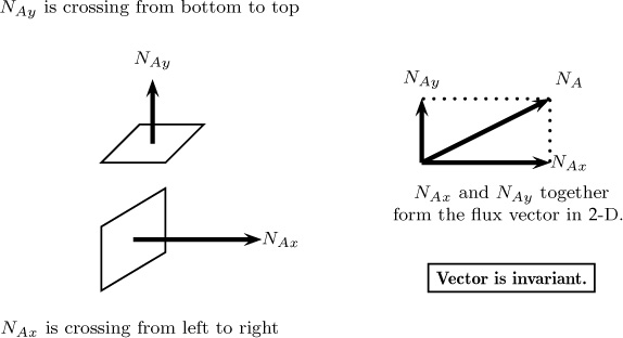
Figure 1.1 Notion of flux vector and representation of its components. The flux vector is uniquely defined as any given point, while the components depend on the constructed coordinate system. Thus, if the coordinates are rotated, the components will be different but the flux vector will be the same.
If we use the mass units, we can define a mass flux vector, which is usually denoted as nA, with the units being kg A/m2 s.
The flux vector is unique at a given point, whereas the components NAx and so forth depend on the orientation of the x-axis and other dimensions. Thus the components can change in magnitude if, for example, the coordinates are rotated. This will not alter the results in any way since the flux vector is frame indifferent. Similarly, the flux components can be defined in cylindrical, spherical, or other body-fitted coordinate systems and used for the specified geometry. The flux results both from diffusion and due to the flow rate across the control surface and hence the flux are referred to as combined flux. For modeling purposes, it is necessary to split this entity into diffusion flux and convection flux. Thus
Combined flux = convection flux + diffusion flux
This partitioning, which is illustrated in Figure 1.2, is not unique. Rather, it will depend on which value is assigned to the convection flux, as will be shown in the next section.
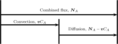
Figure 1.2 Partitioning of the combined flux into diffusion and convection flux. The total flux is fixed from the conditions prevailing at that point. In contrast, the partitioning is not unique and depends on the definition of the mixture velocity, v.
1.3.2 Convection Flux
Convection is transport due to flow, and convection flux can be easily calculated if the velocity of flow is known. Thus, if there is a velocity vx in the x-direction, then a flux of vxCA results from this velocity in the x-direction and is referred to as a convection flux. In general, for the 3-D case the convection flux depends on (a suitably defined) mixture velocity v and is defined as
Convection flux vector = vCA
Note that the mixture velocity in a multicomponent system is not uniquely defined, unlike in a single-component system. This topic is discussed further in Chapter 5. The point to note here is that the convection flux depends on which definition of the mixture velocity is used. The diffusion flux is correspondingly adjusted since the total flux at any point is fixed.
1.3.3 Diffusion Flux
Diffusion is a tendency for a system to approach equilibrium conditions. This can be considered as a result of molecular-level motion when looked from a continuum point of view. Diffusion is therefore also referred to as molecular transport. It must be modeled based on empirical observation, with the resulting model being called a constitutive model. This result is system specific, as there is no universal law to describe the process of diffusive mass transfer. However, it is common to model diffusion by Fick’s law, which states that the (molar diffusive) flux of A is proportional to the concentration gradient of A, dCA/dx:
Here JAx is the diffusion flux of A in the x-direction. Note that the law implies that the diffusion occurs in the direction of negative concentration gradient— that is, from a region of higher concentration to a region of lower concentration. This is similar to heat flowing from a hot body to a cold body. The constant of proportionality DA is called the diffusion coefficient of A. It has the units of m2/s.
More generally speaking, the gradients in the chemical potential can be viewed as causing mass transfer, such that use of these concepts leads to more complex expressions for the diffusive flux. These complexities are addressed in Chapter 7. One consequence of such models is that DA may not have a constant value over the entire concentration range, but rather may be a function of concentration, especially for a non-ideal liquid mixture. Another consequence is that in some cases, the diffusion can occur counter to the direction of negative concentration gradient. These complex effects and models of them will be deferred to Chapter 7.
Note: A more precise definition of diffusion flux is provided in Chapter 5 and requires a more precise definition of the velocity of a multicomponent mixture. The point to note at this stage is that in a multicomponent system, the mixture velocity is not uniquely defined, unlike in a single-component system. The diffusion flux is defined correspondingly, with the mixture velocity as the frame of reference. Also, Fick’s law (shown by Equation 1.12) applies to a system in which the total concentration C remains constant at various points in the system. A more general representation and the topic of diffusion in systems with total constant density are deferred to Chapter 5. Nevertheless, for many applications the simple Fick’s model for diffusion shown here is widely used.
Generalization of Fick’s law to the 3-D case is accomplished by using the notion of the gradient of a scalar:
where ∇CA is the concentration gradient vector.
Typical Values of Diffusivity
The range of values of the diffusion coefficient depends on the phase in which transport is taking place. The range of values are shown in Table 1.1.
Table 1.1 Order of Magnitude Values of the Diffusion Coefficient
System |
DA Values in m2/s |
Gas in gas |
10–5 to 10–4 |
Gas in porous solid |
10–6 to 10–5 |
Gas in narrow pores |
10–8 to 10–6 |
Liquid in liquid |
10–10 to 10–9 |
Liquid in porous solid |
10–11 to 10–10 |
Solid in solid |
10–12 to 10–17 |
Note that the convection flux is proportional to the concentration, while the diffusion flux is proportional to the concentration gradient.
Although convection and diffusion are the two fundamental modes of mass transport, additional phenomena such as turbulent diffusion and dispersion are also used. These are not independent mechanisms, but rather reflect the combined effects of diffusion and convection. A brief description is provided here, but detailed discussion of these topics is deferred to later chapters (4 and 12).
Turbulent Diffusion
Convective transport is due to fluid motion. Fluid flow can be either laminar, turbulent, or transitional, depending on the flow rate, viscosity, and other parameters. For steady-state laminar flow, the velocity is time independent and the convection flux based on the time-independent velocity applies. However, in turbulent flow, random fluctuating components of velocity are superimposed on the main flow. The convective mass transport due to the fluctuating part of velocity, when averaged over time, is usually modeled as an additional mode of transport, referred to as eddy diffusion or turbulent diffusion. Thus the turbulent diffusion is a consequence of the concept of time averaging widely used in study of turbulent transport and is not an independent mass transport mechanism.
Diffusion can be viewed as manifestation of random molecular motion, while turbulent diffusion can be viewed as the result of random bulk motion of the eddies. Diffusion brings in species from a region of higher concentration to a region of lower concentration. Similarly, turbulent eddies bring in species from a region of higher concentration to a region of lower concentration and the process can be modeled by an equation similar to Fick’s law:
where Dt is the turbulent diffusivity, also known as eddy diffusivity. Turbulent diffusivity is a flow-dependent property rather than a molecular property. The is a time-averaged value of the fluctuating concentration, which is a characteristic of turbulent transport. Models to calculate Dt are provided in Chapter 12. (This quantity is commonly defined as the time average of the product of velocity fluctuation and the concentration fluctuation.)
Dispersion
Consider the flow of a fluid in a pipe. There is a velocity profile across the tube radius. The velocity at the wall is zero, while that at the center is at its maximum. The contribution of the convection resulting from this velocity profile and the associated diffusion, when averaged across the pipe cross-section, can be modeled as another mode of mass transfer, referred to as dispersion. Thus the dispersion is a consequence of the concept of cross-sectional averaging, which is widely used in mesoscopic model analysis (described in more detail in Chapters 4 and 14) of mass transport, rather than an independent mass transport mechanism.
1.4 Concentration Jump at Interface
Another important point to understand is that the concentration is not continuous at a phase boundary (e.g., gas–liquid interface), unlike temperature. Consider air–water system as an example. Is the oxygen concentration on the air side of the interface the same as the oxygen concentration on the water side of the gas–liquid interface? The answer is no. Because oxygen has a poor solubility in water, the oxygen concentration in the water phase in much lower than that in the air phase. This difference in concentration is called the concentration jump at the interface. The thermodynamic relations needed to calculate the jump are for various cases are discussed next.
1.4.1 Gas–Liquid Interface: Henry’s Law
The concentrations on the gas side and on the liquid side of the interface are often assumed to be linearly proportional—a concept summarized by Henry’s law. The constant of proportionality is known as the Henry’s law constant. Various definitions are used for this constant, depending on the units used to measure the concentrations. The common form is as follows:
where pA is the partial pressure of the species in the gas phase and xA is the mole fraction in the liquid. The constant HA has the units of atm or Pa or bars here. The values of the Henry’s law constant for some common gases are shown in Table 1.2.
Table 1.2 Henry’s Law Constant for Some Common Gaseous Species in Water at 298.15 K
Gas |
H, atm |
Hydrogen |
7.099 × 10⁴ |
Oxygen |
4.259 × 10⁴ |
Nitrogen |
8.65 × 10⁴ |
Ozone |
4570 |
Carbon dioxide |
1630 |
Sulfur dioxide |
440 |
Ammonia |
30 |
The larger the value of the Henry’s law constant, HA, the less soluble the gas is in the liquid phase. The effect of total pressure in the system is to increase the solubility in accordance with Henry’s law. In general, increasing the temperature decreases the solubility. Hence the Henry’s law constant is usually an increasing function of temperature. An exception occurs with hydrogen, which shows a retrograde behavior. Here the solubility increases at first with an increase in temperature, reaches a maximum, and then decreases thereafter.
Other Definitions of Henry’s Law Constant
Other definitions of the Henry’s law constant are also used, depending on which unit is used for the concentrations in the two phases. Two common definitions are as follows:
where HA,pc is the Henry’s law constant (unit of Pa m3/mol) with partial pressure, Pa, as the unit for the gas phase and mol/m3 as the concentration unit for the liquid phase, respectively. Another form is
where HA,cp is the Henry’s law constant (unit of mol/Pa m3) and is the reciprocal of HA,pc.
Since the concentration in the gas phase can also be used instead of the partial pressure unit, we have yet more ways of writing the Henry’s law relationship! Example 1.1 shows the application of the Henry’s law and the concentration jump at a gas–liquid interface.
Example 1.1 Oxygen Concentration in Water
Find the dissolved oxygen concentration in water, assuming equilibrium conditions.
Solution
Let A represent the oxygen species. The mole fraction in the liquid is then calculated using Henry’s law:
xA = pA/HA = 0.21 atm/4.259 × 104 atm = 4.963 × 10⁻⁶
Hence the concentration in the liquid is xAC, where C is the total concentration of the liquid mixture. For dilute systems, C is simply the solvent concentration. For water, the density is 1000 kg/m3 and the molecular weight is 18 × 10–3 kg-mass/g-mole. Hence
C = 1000/(18 × 10–3) = 55, 560 mol/m3
The oxygen concentration in the liquid is therefore 0.2739 mol/m3. If air is bubbled for a long time in a batch of liquid, the oxygen concentration in the entire liquid will reach the previously given value, which is the final equilibrium value.
To illustrate the concentration jump at the interface, we can also calculate the concentration of oxygen in air using the ideal gas law:
CAG = yAP/RgT = 0.21 atm * 1.01 × 105(Pa/atm)/8.314/298 = 8.467 mol/m3
The ratio of CAG to CAL is 30.9, which is the magnitude of the concentration jump at the interface.
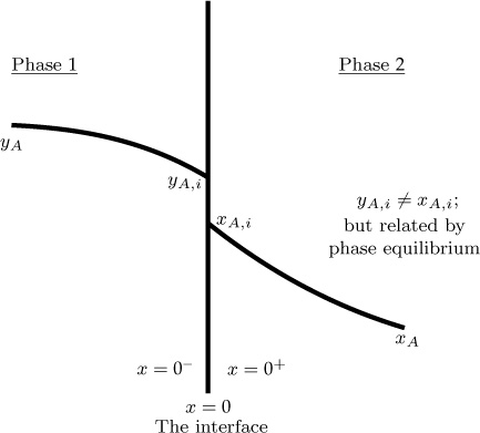
Note: Mass transport is usually performed under non-equilibrium conditions. Hence Henry’s law should be applied only at the interface, which is assumed to still be at equilibrium. Concentrations in phase 1 and phase 2, away from the interface, will not be the equilbrium values. Otherwise, no mass transfer will occur.
The schematic of the concentration variation for interfacial mass transfer is shown in Figure 1.3. Although the concentration varies in both phases, the interfacial concentration values are related by thermodynamic considerations. The subscript i in Figure 1.3 refers to the interface and yAi and xAi are related by Henry’s law.
1.4.2 Vapor–Liquid Interface: Raoult’s Law
For volatile liquid-phase species, Raoult’s law is often used to relate the interfacial concentrations. It states that at the vapor–liquid interface, a pure liquid exerts a partial pressure equal to the vapor pressure of the liquid at that temperature. For an ideal liquid mixture, the partial pressure at the interface is equal to the vapor pressure multiplied by the mole fraction in the liquid. Hence the interfacial relation is
pA,i = xA,i pvap,A
The vapor pressure pvap varies as a function of temperature and is often correlated by the Antoine equation:
Values of the constants A, B, and C are tabulated in many books (for example, Reid et al., 1987) and websites. The units are often in mm Hg for vapor pressure and temperature (T) is in degrees Celsius rather than in standard S.I. units. Hence caution must be exercised when extracting these values from the literature.
1.4.3 Liquid–Liquid Interface: Partition Constant
A simple partition constant (denoted as mA for species A) is often used to describe the interfacial equilibrium between two liquids:
yA,i = mAxA,i
where yA,i is the interfacial mole fraction in one of the liquid phases and xA,i is the interfacial mole fraction at the interface of the second liquid. The partition coefficient, in turn, is related to ratio of activity coefficients of A in the two phases:
The value of this coefficient is often predicted using thermodynamic models for activity coefficients.
1.4.4 Fluid–Solid Interface: Adsorption Isotherm
Thermodynamic jump at gas–solid or liquid–solid interfaces is defined in a similar manner, using an adsorption equilibrium constant that has a same status as the solubility or partition coefficient. Often a linear relation is used: qA = KACA where qA is the equilibrium concentration of A in the solid phase and CA is its concentration in the gas phase. KA is referred to as the (linear) adsorption equilibrium constant.
1.4.5 Nonlinear Equilibrium Models
A note is in order regarding the linear models described in the previous sections. These models are widely used, even when they do not hold exactly for simplification of the models. However, more complex models are needed to describe equilibrium in non-ideal liquid mixtures—and in systems where there is a strong adsorbed layer due to differences between the interfacial tensions of various species dissolved in the liquids. This layer often has completely different property from the two liquids in contact and is sometimes referred to as a microphase.
On a similar note for fluid–solid systems, linear adsorption equilibria are often used, although these are actually the limiting case of nonlinear relations (the classical Langmuir equation and other isotherms are described in Section 29.3). The linear relation is a good approximation for dilute systems. More generally, the Langmuir isotherm is used to represent equilibrium for gas–solid and liquid–solid systems for concentrated solutions. For gases that undergo a reaction in the liquid, the solubility has to be viewed as the first step for the dissolution equilibrium constant—for example, A(gas) to A(aq) equilibrium. Dissolved gas may further react; hence the quantity of gas absorbed will also depend on the equilibrium constant for these reactions, which are accounted for separately. This value can exceed that calculated using the solubility parameter alone. An example of such system is SO2 in water, where the dissolved SO2 undergoes reaction to form or ions depending on the pH of the solution.
1.5 Application Examples
Mass transport processes are ubiquitous in nature and engineering practice. One can cite numerous examples, which by themselves will fill an entire book. This section presents a few examples and includes the questions that an engineer may ask in an attempt to understand or design these processes. As the content of this book unfolds, we will be in a position to answer these questions and perhaps raise yet more questions. As you will appreciate from a perusal of these examples, the analysis and modeling of mass transfer processes (the main goal of this book) is widely useful in many fields. You will be well trained to tackle problems in your chosen engineering profession and be in a good position to do research and advance this area upon completing your study of this book.
1.5.1 Reacting Systems
Heterogeneous reactions are commonly encountered in chemical processing. These systems include two or more phases, with reaction taking place mainly in one of the phases while the reactants are usually present in the other phase. Hence a prerequisite for reaction to occur is mass transfer from one phase to the other. This coupling of mass transfer and reaction has many interesting consequences, which are studied in detail in Part II of the book. A simple classification of heterogeneous reacting systems is based on the type and number of phases contacted, as shown in Table 1.3 (along with one example for each case). Most reaction engineering books include sections on heterogeneous reactions and offer varying degrees of coverage of this area (e.g., Levenspiel, 1974). The extensive (almost encyclopaedic) monograph by Doraiswamy and Sharma (1984) is an useful reference book and deals exclusively with heterogeneous reactions.
Table 1.3 Examples of Heterogeneous Reactions Based on the Phases Being Contacted
Phases Contacted |
Example |
Gas + solid catalyst |
oxidation of ethylene |
Gas + solid reactant |
combustion of coal |
Gas–liquid |
removal of CO2 by reactive solvent |
Liquid–liquid |
biodiesel production |
Gas–liquid + solid catalyst |
removal of sulfur compounds from diesel |
Gas–liquid + solid reactant |
carbonation of lime |
Gas–liquid–liquid |
production of hydroxylamine from nitrobenzene |
Two examples of reacting systems where mass transfer plays an important role are shown here. Other examples are taken up in Part II.
Catalytic Converter
A common example of mass transfer accompanied by reaction is found in an automobile. A catalytic converter consists of a set of flow channels coated with an active layer of catalyst such as platinum (Pt). This is an example of a flow system accompanied by mass transfer and chemical reaction to reduce the release of pollutants such as CO and NOx. The extent of pollutant removal depends on the flow rate of the gas, the temperature, the rate of mass transfer to the catalytic surface, and the rate of the reaction at the surface itself. The overall rate of reaction can be calculated by a mass transfer analysis and used to design the converter. The dynamic response of the system and the extent of pollutant removal during the initial cold start period (when the converter is cold) can also be found using these models.
Trickle Bed Reactor
A trickle bed reactor is an example of a three-phase reactor (gas–liquid–solid catalyst). It is similar to the packed column used in the unit operation of absorption of a gas. Here gas and liquid flow over a packed catalytic bed and a reaction occurs on the surface of the catalyst (Figure 1.4). Gas, liquid, and solid catalyst are the three phases present in the reactor. Such reactors are widely used in the chemical and petroleum industry. For example, they are used to remove sulfur compounds from diesel, an application that relies on a reactor with three phases: hydrogen, diesel, and a cobalt–molybdenum (Co-Mo) based catalyst. Today’s urban air is often cleaner thanks to the trickle bed reactor. The book by Ramachandran and Chaudhari (1983) is a good starting source on this subject and covers the various types of three-phase catalytic reactors in detail.
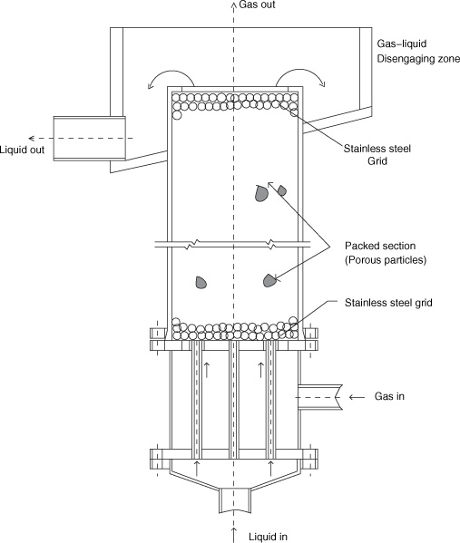
Figure 1.4 Schematic of a trickle bed reactor; mass transfer of species in the gas phase (e.g., hydrogen) to the liquid and then to the surface of the catalyst is followed by a surface reaction on the catalyst with a second species diffusing from the liquid. (An operation with upflow of both phases is shown here.)
1.5.2 Unit Operations
Unit operation is defined as a unified study of a particular separation technique used for a chemical engineering application. Distillation is an example in which the vapor pressure differences between two components are used to separate and purify these components. The unit operation approach takes the view that the analysis is same whether you are doing a distillation of a crude oil mixture or making brandy. Common mass transfer–based separation processes are listed in Table 1.4. All of these separations rely on interfacial mass transfer; hence the analysis and modeling of mass transport effects is a prelude to the design of such systems.
Table 1.4 Common Mass Transfer–Based Separation Processes and the Phases Being Contacted
Phase 1 |
Phase 2 |
Operation |
Vapor |
Liquid |
Distillation |
Gas |
Liquid |
Absorption |
Liquid |
Gas |
Stripping |
Liquid |
Liquid |
Extraction |
Gas |
Solid |
Adsorption |
Liquid |
Solid |
Adsorption |
Wet solid |
Gas |
Drying |
An example of a unit operation is liquid–liquid extraction. The schematic of a simple single-stage extraction unit is shown in Figure 1.5, and we will use this unit as a prototype example for modeling stage contactors. In this unit operation, two phases are intimately mixed in the mixer section of the contactor to create an emulsion or dispersion, which promotes a high rate of mass transfer. The two-phase mixture is then allowed to settle in the settler section, and the enriched solvent and the lean solutions are separated. Determining the degree of mass transfer that can be achieved for a specified rate of agitation is one of the objectives of the mass transfer calculation.
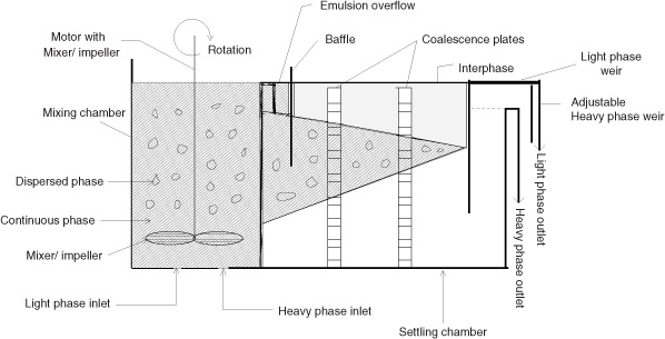
The degree of separation that can be achieved in a single-stage contactor is usually limited; hence a multistage cascade is used, with the lean solution being treated further with fresh or recycled solvent. A designer may want to know how many stages are needed to achieve a certain level of purity. Modeling of such a multistage cascade is used to provide the answer.
Part III of the book covers the application of mass transfer principles to design some of the various unit operations listed in Table 1.3. The key idea is that the modeling methodology is common to all the unit operations and can be approached in an unified format. Thus the various aspects of individual unit operation, although very important on their own, can be brought together under one umbrella of modeling of mass transfer processes. Seader, Henley, and Roper (2011) offer valuable insights into separation process principles and provide a detailed analysis of the various operations.
1.5.3 Bioseparations
Bioseparation refers to separation of products produced by biochemical reactions; the separation of products from a fermentation broth is an often-cited example. These processes have a number of distinguishing features compared to the traditional separations practiced in the bulk chemical and petroleum industry. The distillation is the main workhorse in the chemical industry, but due to the heat-sensitive nature of bioproducts many alternative separation methods are needed. Rapid extraction may also be a requirement since the product may degrade or react further (e.g., in penicillin separation). In many cases the compounds may be present in low concentrations. The target compound to be separated may have similar properties to the other compounds in the broth, so that novel separation tools are needed. Common techniques used are extraction, adsorption, chromatography, and electrophoresis, and the use of mass transfer analysis for modeling these cases is illustrated in later chapters.
The book by Harrison, Todd, Rudge, and Petrides (2003) is a good introduction to this field. The book by Seader et al. (2011) has also considerable information on this topic. A review article published by Harrison (2014) provides an introductory reading, with the author stressing the importance of understanding the basic principles and theory as a prelude to design and control of purity of products obtained in bioprocessing.
1.5.4 Semiconductor and Solar Devices
The heart of the computer you use is made of a silicon chip, but the electronic activity arises due to the fact that the chip has undergone a diffusion process to incorporate phosphorus, boron, or other dopants. Semiconductor doped with group V metals are called n-type, while those with group III metals are called p-type. A junction is formed by contacting these two types of semiconductors and acts as a diode or transistor. The electronic behavior in such systems depends on the transport of the electrons from the n to p side and transport of holes from the p to n side, together with recombination. The diffusion-reaction analysis for porous catalysts presented in Chapter 18 can be readily adapted to this system.
A number of processing steps in this field involve chemical vapor deposition, in which a species (precursor) is transported from a vapor and reacts and forms a deposit or a film on a (substrate) surface. This process again involves mass transport of reactants, with control of the deposited material’s properties being affected by the rate of transport. Oxidation of silicon to form an insulating layer is another example of mass transfer in fabrication of metal oxide semiconductor (MOS) devices. The book by Middleman and Hochberg (1993) is a classic in this area and a must-read for students who wish to get involved in this field.
1.5.5 Biomedical Applications
The focus of mass transfer analysis in the field of biomedical engineering is to bring together fundamentals of transport models and life sciences principles. Key areas where mass transport phenomena can be utilized include the following:
Pharmacokinetics analysis, distribution, and metabolism of drugs in the body
Understanding of transport of oxygen in the lungs and tissues
Tissue engineering, including development of artificial organs
Design of assistive devices such as dialysis units
Some application examples are briefly described in this book in Chapter 23. An early book by Lightfoot (1974) and the more recent books by Sharma (2010); Truskey, Yuan, and Katz (2004); and Fournier (2011) are illustrative of the mass transport applications in this field.
1.5.6 Application to Metallurgy and Metal Winning
Transport phenomena analysis and models are widely used in metallurgy and metal winning. Books by Szekely and Themelis (1991) and by Geiger and Poirier (1998) provide a number of applications in this field. Ore smelting in a blast furnace, gas–solid reactions in steel and copper making, and alloy formation by melt drop solidification are examples of applications in which mass transport principles are needed. Electrochemical processes are also used for metal winning (e.g., copper), in which transport of copper ions to the cathode is an important step in the overall process.
1.5.7 Product Development and Product Engineering
Transport phenomena are increasingly being exploited in product development. Example applications include the design of drug capsules that should provide a constant release rate and the design of polymer wrapping in food packaging to reduce oxygen diffusion. The book by Cussler and Moggridge (2001) is an useful resource for further reading in this field.
An example of drug release from a capsule is shown in Figure 1.6. In this case, if the drug has a uniform concentration inside the capsule, the release rate reaches its maximum in the beginning and decreases with time. Ideally we want a (nearly) constant rate, like that shown in the figure. The design of the pore structure of the capsule to achieve this type of steady release rate is an important application of transient mass diffusion principles.
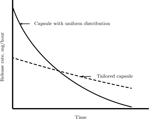
Figure 1.6 A product design application example. The drug release rate is shown for a drug with both a uniform distribution and a tailored capsule.
1.5.8 Electrochemical Processes
Electrochemical processes have a wide range of applications, including batteries, solar cells, electro-deposition, thin films, and microfluidic devices. Transport phenomena principles are increasingly being used to design and improve these kinds of devices. The book by Newman and Thomas-Alyea (2004) is a good treatise on this subject.
In the energy sector, there is a need to store solar energy generated during nonpeak hours and to develop improved batteries for electric cars. A commonly used type of battery is the lithium-ion battery shown in Figure 1.7. Here Li ions are transported across the electrolyte separating cathode and anode. During the charging cycle, Li ions are transported and stored in the carbon matrix. During the discharging cycle, the transport takes place in the opposite direction, such that Li is stored in the metal oxide matrix. Mass transport considerations are an important component in the simulation of the performance of this device; a mass transfer–based model for this system is discussed in Chapter 24.
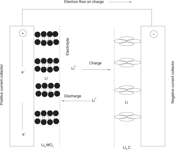
Figure 1.7 Schematic of a lithium-ion battery showing the various mass transfer and reaction steps occurring in the equipment. Lithium ions stored in the carbon “hotels” are released during the discharge cycle and diffuse through the electrolyte to the cathode, where they react with metal oxide matrix. This produces a current in the external circuit.
1.5.9 Environmental Applications
Transport phenomena principles and modeling have found extensive applications in environmental engineering, where they provide a modern perspective and new approach. Typical environmental problems that may addressed using the transport modeling methodology are as follows:
Fate and contaminant transport in the atmosphere is usually simulated by dividing the system into four (air, water, soil, and biota) or more compartments and considering transport and reaction in each of the compartment. See, for example, Figure 1.14.
Groundwater transport is another example. Leakage of contaminants from nuclear waste tanks into rivers could be a major problem, and some of these scenarios can be analyzed by transport models to provide information on the rate of leakage and measures needed to alleviate the problem.
Transport of excess nutrients to water bodies leads to algae growth and destruction of other organisms, a process known as eutrophication. The rate of transport in such systems is needed to determine further remediation actions.
Carbon dioxide sequestration in underground mines is contemplated as a solution to reduce the impact of global warming. Mass transfer analysis is needed to predict the leakage and long-term feasibility of this solution.
The book by Clark (1996) provides a nice introduction to some of the problems mentioned here.
Next, we discuss the general methodology involved in setting up models for mass transfer processes.
1.6 Basic Methodology of Model Development
In this section, we discuss the basic procedure for developing mass transfer models. The starting point for model formulation is to choose a control volume and mark its boundary surface (i.e., the control surface). A system or control volume can be defined as any part of the equipment, as the entire equipment, or even as the large-scale system as a whole. The basic conservation laws are then applied to the system. Conservation law is discussed in Section 1.7.
Control volume can be of any size and shape. Typically, models at three levels are developed based on the size of the control volume: differential models, macroscopic (or macroscale) models, and mesoscopic (or mesoscale) models. These three types of models are explained sequentially in the following sections. On the topmost level is the differential control volume and the differential models. This type of model contains the local information at each point in the continuum. However, for design of process equipment, macro or meso levels may also be used. Although models at these levels are not as detailed as the differential models, they are easier to solve and to apply in practical designs. Hence modeling at all three levels is covered in this book.
For modeling very large or complex systems, such as transport of a pollutant in the environment or drug metabolism in the human body, the system is divided into a number of interconnected compartments and a macroscale model is applied to each compartment. Applications of these so-called compartment models are provided in Chapter 13.
Conservation laws alone are not sufficient to complete the model, since the model will contain terms for the mass crossing into a control surface. Hence additional closure relations are needed. For example, a differential model using the conservation principle alone will contain the flux vector as a parameter. This system has to be closed and a flux versus concentration relation has to be applied using a constitutive model. Similarly, the macro- and meso-level models may contain terms such as the mass crossing a larger-size control surface or from one phase to another. Suitable transport laws must be applied to close these terms, thereby completing the model. Hence coupling the conservation laws together with suitable transport law is the basic methodolgoy in developing mass transfer models.
1.7 Conservation Principle
The conservation principle is the consequence of the law of mass conservation, which states that a species A cannot appear from nowhere and must be conserved. The species mass balance is therefore the starting point:
Species A can cross into the control volume from a part of the control surface (the in term) and leave out of the rest of control surface.
Species may also be consumed (depletion) or produced (generation) within the control volume by chemical reaction.
Finally, the species concentration in the control volume may change with time due to the accumulation of the species within the control volume. The various processes involved are shown schematically in Figure 1.8.
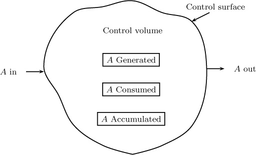
The depletion is normally taken as a negative generation term and is often not included separately. In such cases, the generation is to be understood as net generation, which is equal to generation – depletion.
Similarly the out – in term is often written as a net efflux term. Hence another form of the conservation statement is
(Net) Generation = Net efflux + Accumulation
We now illustrate the use of this principle for the three levels of models discussed earlier and indicate which additional relations are needed to complete the model.
1.8 Differential Models
In differential models, a differential control volume (e.g., a box with sides Δx, Δy, and Δz for Cartesian coordinates) is used to develop the transport models. The control volume is then made to tend to zero, thereby producing a set of differential equations for the primary field variable—namely, the concentration. These equations represent models at the highest level of hierarchy and contain the detailed information.
The simplest differential control volume is the one constructed in Cartesian coordinate volumes, which is shown in Figure 1.9. The net generation and accumulation depend on the control volume and, therefore, are known as volumetric terms. The net efflux term, known as the surface term, depends on the combined flux at that control surface. Application of the conservation principle, then, leads to the species mass balance equation involving the unknown fluxes. Nevertheless, this equation alone is not sufficient: We need additional relations because we ultimately want to solve for the concentration field. The flux term in the equation is the combined flux, which is the sum of the convection flux and the diffusion flux. The convection flux depends on the local velocity and local concentration, so it can be calculated if the velocity profile in the system is known. The diffusion flux results from the molecular interactions, which are not modeled at the continuum level. Hence a closure equation—that is, a constitutive model for diffusion— is needed to close the model. The most commonly used constitutive model is some form of Fick’s law. Note that for multicomponent diffusion in mixtures, the Stefan-Maxwell model for diffusion is also used; it is discussed in detail in Chapter 15.
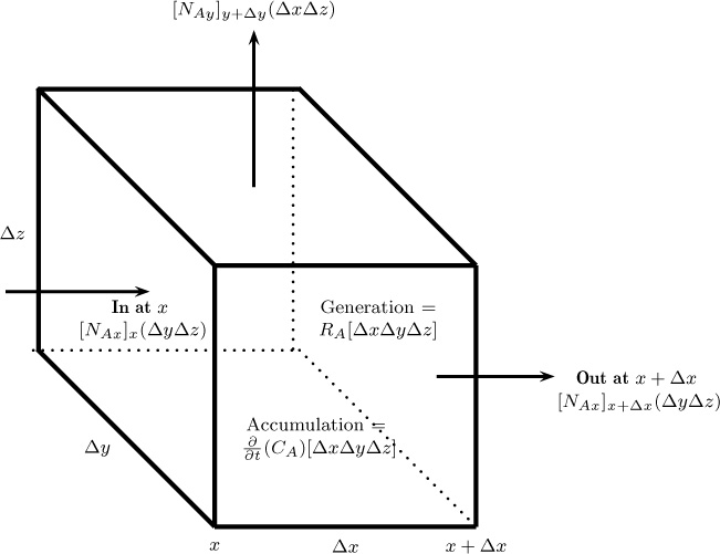
Figure 1.9 Differential control volume in Cartesian coordinates. Note: Flux components from the hidden faces are not shown to avoid clutter.
In summary, mass transfer models at the differential levels are built through the combination of the conservation law and the constitutive law. The differential equations of mass transfer based on this approach are derived using this methodology in Chapter 5 and have general applicability. Many simpler problems can be deduced by simplification of these equations. In essence, this method is similar to that used in fluid mechanics, where the Navier-Stokes equations have general applicability for modeling flow of Newtonian fluids and where solutions to specific problems such as pipe flow can be obtained by simplification of these general equations. Likewise, we can go from the general to the particular in modeling of mass transfer. However, for simpler cases where the concentration varies only along one coordinate direction, it is instructive to derive and solve the equation by starting directly from the conservation laws and then using Fick’s law, rather than by directly using the general differential equations. This approach is illustrated in Chapter 2 for some common problems in mass transfer. A careful study of Chapter 2 will provide you with a basic understanding of the process of setting up and solving differential models.
1.9 Macroscopic Scale
At the macro-level of modeling, a large-size control volume or the whole equipment is used. The conservation laws are, in turn, applied to this region. The volume element is not taken to tend toward zero, and the balances based on the selected larger volume are used directly. Such models are useful to obtain the relation between engineering quantities in an approximate way. Point-to-point information (details) is lost at this level, however, and the effects of these variations have to be incorporated through some sort of calculation (model averaging followed by some approximations) or by other means (e.g., empirical fitting of experimental data). This leads to the information loss principle:
Information, on length (or time) scales lower than that at which analysis is done, is lost and has to be supplemented in some suitable manner.
Appreciation and awareness of this principle are important in modeling. In particular, for the macroscale analysis discussed in this section, we lose information on the point-to-point concentration values and the point-wise variation of the flux over a given control surface. This loss must be countered by making some assumptions and using some closure models. In the following sections we discuss qualitatively the closures commonly used by examining some specific examples. More fully worked-out examples of macroscopic balances are provided in Chapter 3 and continued in Chapter 13.
1.9.1 Stirred Tank Reactor: Mixing Model
Consider a reactor that is stirred and operated continuously with in and out flows of a liquid. The control volume is the whole reactor shown in Figure 1.10; the various contributions to the mass conservation are also shown in a general manner in this figure. Now assume the reactor consists of a single phase and is operating at steady state. The accumulation term is zero. The loss term for the second phase shown in the figure can also be neglected here if we have only one phase. The conservation law simplifies to
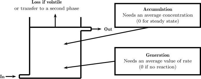
Figure 1.10 Illustration of a macroscopic control volume showing the various components that go into the species balance. The average values are the integrals of the (unresolved) pointwise values. The information on the pointwise values is lost at the macro-scale modeling level. Hence model assumptions or closures are needed.
in – out + generation = 0
where all the terms are in moles A per unit time.
Now let’s use mathematical terms to describe this system. In and out can be formulated in terms of the volumetric flow rate times the corresponding concentration. The main assumption needed is for the generation term. This term is the total generation over the entire control volume and is the volume integral of the local rate of reaction (mole/m3 local volume sec) RA. The local rate, in turn, is a function of the local concentration. We assume that the required relation is known from a kinetic model. Now the generation over the entire volume is the volume integral of the local rate:
Here RA (local) is some specified function of the local or pointwise concentration.
This local concentration is not known (not being modeled) in the macroscopic model, so it is not possible to evaluate precisely the generation term. Hence some assumption about the mixing level in the reactor (the concentration variation in the reactor) must be made. These details are studied in Chapters 3 and 13.
A common simplifying assumption is that the reactor is well mixed and the reactants present at a uniform concentration. This permits us to close the model, which is then referred to as a completely backmixed model. Many other models for closure may be used depending on the anticipated mixing level in the system (e.g., dividing the tank into a mixed zone and a dead zone or dividing the tank into two well-mixed subcompartments), and some of these models are explained in more detail in Chapter 13. The main point to note here is that some assumption about the mixing pattern must be made and the level of mixing needs to be tested and quantified by suitable experiments (e.g., by tracer methods).
1.9.2 Sublimation of a Solid Sphere: Mass Transfer Coefficient
Consider a solid that exerts sufficient vapor pressure and is subliming into a gas phase. The change in the radius of the solid is to be computed. A macroscopic balance for the solid is in order. In is zero and out is the mass transferred from solid to gas. In this scenario, the conservation law for the solid simplifies to
in (zero) – out (transferred from solid to gas) = accumulation
The rate of transfer from solid to gas is precisely the surface integral of the radially directed outward flux at the surface of the solid:
where NAs is the radial component of the flux vector at the surface.
This flux vector can be computed only if a differential model for the gas phase is solved, including the convection and diffusion of the solute in the gas phase. It is not always possible to do this (or such details may not be important) since this endeavor is computationally intensive and the velocity profile in the gas phase may not be precisely known for complex geometries and for turbulent flow. Obviously, we need a closure for the unknown term, which done by introducing the mass transfer coefficient, km. Using this parameter, we model the transfer rate as a product of the mass transfer coefficient times a concentration difference:
CAs – CAb is taken as a driving force for mass transfer from the solid to the bulk gas. Note that CAs is the concentration of A in the gas phase at the gas side of the solid–gas interface, just near the solid. CAb is the concentration in the gas phase at a point far away from the solid, known as the bulk gas. This concentration is usually taken as zero.
Equation 1.19 is actually a definition, rather than a fundamental law. The mass transfer rate is given per unit area of transfer. Balancing the unit, we find that the mass transfer coefficient has the units of m/s. Values of the mass transfer coefficient are provided by numerous sources. For example, they may be empirically fit to experimental data or fit to detailed computational models. For many practical cases the values of the coefficient have previously been published; as a consequence, the concept of the mass transfer coefficient is widely used in practical design calculations. The main point here is that the use of the mass transfer coefficient completes the missing flux information in the context of macro-level (as well as meso-level) models.
1.9.3 Model for Mixer-Settler
Consider the mixer-settler shown in Figure 1.5. There are two phases present in this system: the dispersed phase (drops) and the continuous phase. Obviously, the differential model for both the dispersed and continuous phases is needed for a detailed analysis and can be quite challenging to construct. Here a two-phase flow model together with a local model for interfacial flux needs to be developed. In industrial design, however, macroscopic models are usually the models of choice. Here we assume that there are two control volumes: one for the solvent phase and one for the aqueous phase. These two control volumes have a common interface across which the solute is transferred. In other words, the system is modeled as two interconncected control volumes, one for the aqueous phase and one for the solvent phase. A schematic of such control volumes used in macroscopic analysis of two-phase systems is shown in Figure 1.11. The transfer rate is modeled by using a suitably defined mass transfer coefficient. In addition, we must make an assumption about the mixing pattern in both phases as well as the value for the mass transfer coefficient. For example, are these phases completely mixed? In that case the backmixed assumption is sufficient. Also, how does the mass transfer coefficient change if some design parameter (e.g., agitation speed) is changed? These details needed to design the equipment are explored in more depth in Chapters 3 and 13. At this stage, the various components needed for a macroscale analysis and design of separation equipment simply need to be appreciated.
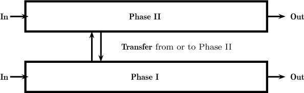
Figure 1.11 Schematic of a mixer-settler for liquid–liquid extraction modeled as two separate but interconnected control volumes.
1.9.4 Equilibrium Stage Model
A simplifying assumption in the mixer-settler model is that the outlet streams are at equilibrium. This will be the case for an ideal contactor in which the mass transfer is complete. Such a simplified model, which is called equilibrium stage model, provides a benchmark for quick design calculations. The actual contactor may not have achieved equilibrium, so the results are often simply corrected by introducing a stage efficiency parameter. This can be an empirically fitted parameter, or it can be computed by including mass transfer effects into the model. Thus we note that a hierarchy of models with increasing levels of complexity can be built for this process—a practice that is common when modeling other separation processes as well. For example, a distillation column can be modeled using (1) a number of ideal or theoretical stages, (2) a number of stages with correction for stage efficiency, or (3) a model based on detailed mass transfer rates.
We now look at mesoscopic models.
1.10 Mesoscopic or Cross-Section Averaged Models
Mesoscopic models are useful when there is a principal direction over which the flow takes place, as in pipe flow, for instance. Control volume is taken as differential in this direction but assumed to span the entire cross-section in the cross-flow directions (Figure 1.12). The rationale for this assumption is as follows: The concentration variation in the flow direction is more significant, meaning it changes significantly from inlet to outlet, rather than in the radial direction. Changes in the radial direction at any fixed axial position may not be very large. Hence the mesoscopic control volume shown in Figure 1.12 is adequate in lieu of a complete differential model. The key point to note is that the information on the radial variation of concentration and its effect of the various terms in the conservation model is lost with this kind of model. Hence an appropriate closure model is needed the supplement the information lost due to area or radial averaging. More details on this approach are provided in Chapter 4. Here, we provide some simple examples of closure models used for this level of modeling.
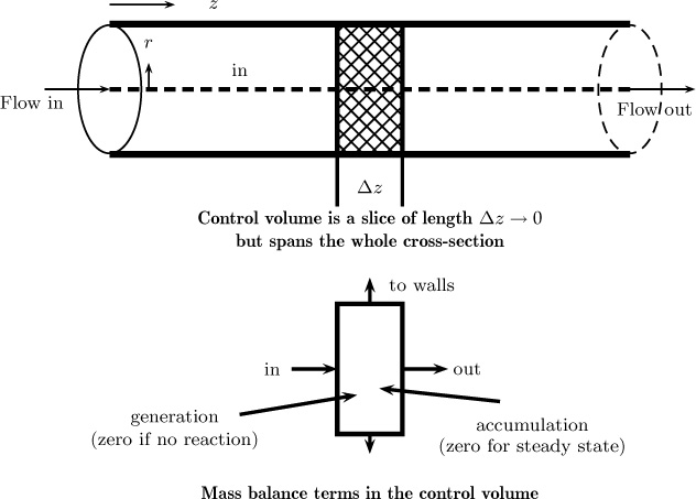
Figure 1.12 Illustration of the mesoscopic control volume for analysis of mass transfer processes in pipe flow. All of the terms in the mass balance are integrals of (unresolved) pointwise values. Hence model or closure for these terms is needed.
1.10.1 Solid Dissolution from a Wall
Consider the mesocopic model applied to a simple system of solid dissolution from a wall in a tube shown in Figure 1.12. Here we have a pipe coated with a dissolving or subliming solute material; a fluid is flowing in the pipe. The concentration of the solute is to be calculated as a function of the length. Two specific examples are a naphthalene-coated pipe with air flow; a pipe coated with benzoic acid (which is a solid at room temperature) with water flow. We assume steady state so that the accumulation is zero.
The conservation law (in – out = 0) is now represented as
in from flow at z + in by transported from the walls –out from flow at z + Δz = 0
To calculate the in and out terms due to flow, we must recognize that the velocity can vary across the cross-section. Concentration also varies along the pipe, with the maximum concentration found at the dissolving pipe wall. The flow can be laminar or turbulent. Laminar flow of a Newtonian fluid has a parabolic profile, whereas the profile is very steep in turbulent flow as shown in Figure 1.13. The velocity for the turbulent flow is the time-averaged value, a concept that is discussed more fully in Chapter 12.
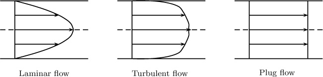
Figure 1.13 Schematic of axial velocity profiles for laminar, turbulent, and plug flow in a pipe as a function of radial position.
A cross-sectionally averaged velocity is an useful quantity and is defined as
which is the integral average of the local velocity. The volumetric flow rate is then equal to 〈v〉 A; v is the axial velocity.
The plug flow shown in the Figure 1.13 is an idealization that is often used to simplify the models. Here the velocity is assumed to be the same at each local radial position. Consequently, the cross-sectional average velocity is also equal to the local velocity.
The in and out terms are the integral average of the axial flux values. The flux component in the axial direction is primarily due to convection and is locally equal to vCA. For a small differential area, ΔA, the moles of A crossing is therefore equal to vCA ΔA. Hence the moles crossing over the entire tube area is the integral of the product of local velocity and the local concentration:
where the notation 〈...〉 is used as shorthand to indicate the averaged value of any quantity within the brackets. Thus we define
We need 〈vCA〉 to evaluate the in and out terms, which cannot be calculated because local concentration values are not available at the meso-level. Hence we define and use an average concentration. This average concentration is called the cup mixing average concentration, of the flow weighted average. It is denoted as CAb and defined as follows:
Hence
The in and out terms are then represented simply as A 〈v〉 CAb. Thus the cup mixing concentration is used as the representative concentration variable in the context of our mesoscopic model. The local concentration has no relevance because the local information is not available. Note: In the context of the meso-level model, the notation CA is used in many books as a simpler notation; by implication, this is the cup mixed average value and should be interpreted accordingly. The results in such models are the variation of the cup mixing concentration with the axial distance.
Example 1.2 shows a calculation of the cup mixing concentration to clarify the definition. Here we assume that the radial variation is known from other methods, such as from a differential model or by experimental measurements.
Example 1.2 Cup Mixing Concentration
A pipe wall is coated with a solute that dissolves into the flowing liquid. The radial variation of the concentration of the dissolved solute in the liquid at a particular axial position was found to be
where CA is the local concentration at radial position r, CAs is the saturation solubility of the solid, and R is the pipe radius. The term cA is the scaled or dimensionless concentration.
Find the center concentration, the concentration near the pipe wall, and the cup mixing concentration. Flow is laminar and the liquid is Newtonian.
Solution
The (dimensionless) center concentration is 1/4 by substitution of r = 0.
The concentration near the wall is equal to 1 by substitution of r = R. Liquid near the wall is saturated, so the dimensionless concentration is one as expected.
The cup mixing is done by using Equation 1.22. The weighting factor of 2πrvz Δr is used in the integral because ΔA = 2πr Δr for a differential annular cross-section. Here vz is the local axial velocity—that is, the velocity at location r. For laminar flow of a Newtonian fluid, this is a parabolic function of r. From fluid dynamics, the following relation is obtained:
Using this information in Equation 1.22, the scaled cup mixing concentration is the ratio of the following integrals:
Having defined the in and out terms using the cup mixing concentration, we need an expression for the transport rate to the walls so as to close the model. This is done by defining and using a mass transfer coefficient. It is common practice to use the cup mixing concentration as the representative concentration away from the solid; the driving force for mass transfer is then defined using (CAb – CAw) as the driving force. Hence the mass transfer rate is defined as
NAw = km(CAb – CAw)
The mass transfer coefficients are available for a large number of flows (such as pipe flows) and, in turn, this approach to modeling is widely used in practice. The mesoscopic formulation can be cast into mathematical framework to account for variation of the concentration (cup mixing) as a function of axial position. Further details and the mathematical details follow in Chapter 4. At this stage, however, you should be able to appreciate the essential concepts that go into the construction of mesoscopic models.
1.10.2 Tubular Flow Reactor
Another common application of the meso-modeling concept is the tubular flow reactor. This is a pipe or channel in which a homogeneous chemical reaction is taking place. We will show that not only the cup mixing concentration is needed, but also another average, the cross-sectional average.
Let us start with the conservation principle in words:
in – out + generation = 0
The generation is the average of the local rate:
generation = (A Δx) 〈RA〉
where
For a first-order reaction, for example, RA = –k1CA, where CA is the local concentration. Hence
To incorporate this into the conservation law, it is customary to define and use the the cross-sectional average concentration:
Hence the generation term (first order) to be used in the reactor model is –(AΔx)k1 〈CA〉.
In and out terms are A 〈v〉 CAb as for the solid dissolution. Thus the conservation law in mathematical terms is
In the limit Δx → 0, this produces the following differential equation:
We find that both the cup mixing and the cross-sectional average appear in the reactor model. Some closure relationship is needed, however, and the commonly used closure models are the plug flow model and the axial dispersion model.
Plug Flow Model
The plug flow model is an idealized reactor model in which the velocity is assumed to be constant, as shown in the Figure 1.13. The cup mixing and the cross-sectional averages are the same since the velocity profile is uniform and, therefore, CAb = 〈CA〉. Only the cross-sectional concentration is needed; that is, no additional closure is needed. Equation 1.26 reduces to
Axial Dispersion Model
The actual reactor may not be a plug flow model, in which case the deviation from plug flow can be modeled by including an additional correction term. The resulting model is known as the axial dispersion model. The representation for the in or out term is
The first term on the right side is the mole flow crossing a cross-section if the plug flow prevails. The second term is a correction term. This system is modeled as though some diffusion type of mechanism is superimposed on the plug flow value. Hence
where DE is called the axial dispersion coefficient. This is only a model, and not a fundamental principle, but nevertheless it provides an important crutch to proceed further in modeling these systems. The axial dispersion coefficient is a commonly used parameter when modeling both reactors and separation processes. Details of the origin of this term and the calculation and application of this concept are discussed in Section 14.2. For now, recognize that the dispersion model closure is
The key points to appreciate from this section are the various definitions and closures that are needed in the context of meso-scale models.
Now we discuss models at an even higher level of simplicity—namely, the compartmental models.
1.11 Compartmental Models
In compartmental models, a set of macroscopic models are interconnected to form a system model for a complicated process. For example, the transport of pollutants in the environment is modeled in this manner. Here it is common to use four compartments as shown in Figure 1.14 to simplify an otherwise complex situation. An application of this model in environmental engineering is described in Chapter 13.
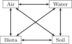
Figure 1.14 Illustration of a compartmental model for pollutant distribution in the environment. Species can be transferred across compartments, as indicated by the arrows. The transfer rate model uses an inter-compartmental exchange parameter.
Compartmental models are also widely used in biomedical systems modeling. A simple two-compartment model to represent the body is shown in Figure 1.15. A simulation example based on this model is provided in Chapter 13.
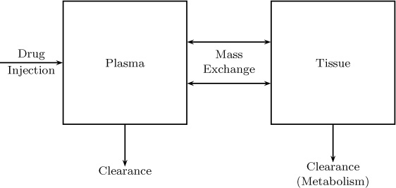
Examples and solutions to compartmental models are taken up in Sections 13.7 and 13.8. It is common practice to simplify each compartment to be a well-mixed system with a constant composition. In addition, an exchange parameter needs to be assigned to model the transfer between the various parameters. In turn, the compartmental models typically use many simplifying (perhaps crude) assumptions. Despite this background, they have proven to have value in environmental and biomedical engineering.
Summary
Mass transport phenomena are ubiquitous in nature and in industrial applications. In essence, the study of mass transfer is the main feature that distinguishes chemical engineering from other engineering disciplines. Mass transfer is caused by diffusion and convection.
Development of a mathematical model to describe a process is central to the analysis and design of a mass transport process. The model is expected to provide information on the concentration in the system and the rate at which a species is transported across the system or equipment.
Analysis of mass transport phenomena is based on the continuum approximation. This assumption permits us to assign a value for concentration at each and every Euclidean point in space.
Concentration can be defined in various ways (mole basis, mass basis, partial pressure, mole fraction, mass fraction), and the relation and conversion from one unit to other should be noted.
An important application of mass transfer is interfacial mass transfer, which refers to the transfer of a solute from one phase to another. For such problems, at a phase boundary (e.g., gas–liquid interface) the values of concentration are different on each side of the interface. This discontinuity is known as the concentration jump at the interface, and thermodynamic phase equilibrium relations are used to close the gaps between the two sides. Hence thermodynamic relations are always needed in the context of interfacial mass transfer.
Models for mass transfer can be developed at many levels. At the topmost level are differential models, which contain the maximum information in the context of the continuum assumption. A differential equation for the field variable, the species concentration, is then developed using the species conservation laws coupled with some constitutive models for transport of mass by diffusion, usually Fick’s law.
Differential models are rather complex to solve for many problems, so models with less details are also used. In general, in transport phenomena analysis, one usually develops model at three levels:
– Differential models provide the most detailed or pointwise information.
– Macroscopic models provide overall information of the system. They typically require some closure parameters on the level of mixing in the system and use of mass transfer coefficients.
– Mesoscopic models provide information on the variation of an averaged property as a function of the main flow direction. The main closure parameters are the transport coefficients and the dispersion coefficient to account for velocity profiles.
The macro- and meso-levels are the volume averaged and cross-sectional averaged description of the differential models, respectively. The definitions of various averages are an important part of the chemical engineer’s vocabulary. The concept of averaging is useful to inter-relate models at various levels of detail.
Compartmental models offer a simplified platform through which to represent complex systems, such as calculation of a drug metabolic process in the human body. These models usually comprise a set of macroscopic control volumes connected in some specified manner.
Review Questions
1.1 What is meant by a concentration jump?
1.2 What is meant by the continuum assumption and what are its implications in model development?
1.3 Indicate some situations where the continuum models are unlikely to apply.
1.4 Give an example of a system in which the total concentration is (nearly) constant.
1.5 Give an example of a system in which the mixture density is nearly constant.
1.6 Can average molecular weight be a function of position?
1.7 Which information is missing in the differential models based on the continuum assumption?
1.8 Why are constitutive models needed in the context of differential models?
1.9 Does the Fick’s law apply universally to all systems?
1.10 Write a form of Fick’s law using partial pressure gradient as the driving force.
1.11 What is meant by the invariant property of the flux vector?
1.12 The combined flux is partitioned into the sum of the convection flux and the diffusion flux. Is this partitioning unique?
1.13 State the units of the gas constant if the pressure is expressed in bar instead of Pa, (ii) if expressed in atm.
1.14 Express the dissolved oxygen concentration in Example 1.1 in parts per million (ppm).
1.15 What is a macroscopic-level model? Which information needs to be added in such a model in addition to the conservation principle?
1.16 How is the mass transfer coefficient defined? Why is it needed?
1.17 What is meant by a cross-sectional average concentration? What is a cup mixing or the bulk concentration?
1.18 Which assumptions are involved in a plug flow model?
1.19 Which assumptions are involved in a completely backmixed model?
1.20 Which additional closure is needed for mass transport in turbulent flow? Why?
1.21 What is an ideal stage contactor? How do you correct the model if the stage is not ideal?
1.22 What is the dispersion coefficient and where is it needed?
Problems
1.1 Mass fraction to mole fractions. Show that mass fractions can be converted to mole fractions by the use of the following equation:
Derive an expression for dyi as a function of dωi values. Do this for a binary mixture. Expression for multicomponent mixture becomes rather unwieldy!
1.2 Mole fraction to mass fractions. Show that mole fractions can be converted to mass fractions by the use of the following equation:
Derive an expression for dωi as a function of dyi values for a binary mixture.
1.3 Average molecular weight. At a point in a methane reforming furnace, we have a gas of the composition CH4 = 10%, H2 = 15%, CO = 15%, and H2O = 10% by moles. Find the mass fractions and the average molecular weight of the mixture. Find the density of the gas.
1.4 Average molecular weight variations. Two bulbs are separated by a 20-cm-long capillary tube. One bulb contains hydrogen and the other bulb contains nitrogen. The mole fraction profile varies in a linear manner along the length of the capillary. Calculate the mass fraction profile and show that the variation is not linear. Also calculate the average molecular weight as a function of the length along the capillary.
1.5 Mass fraction gradient. For a diffusion process across a stagnant film, the mole fraction gradient of the diffusing species was found to be constant. What is the mass fraction gradient? Is it also linear? The mixture is benzene–air.
1.6 Total concentration in a liquid mixture. Find the total molar concentration and species concentrations of 10% ethyl alcohol by mass in water at room temperature.
1.7 Effect of coordinate rotation on flux components. In Figure 1.1, the flux vector is 2ex + ey. Now consider a coordinate system that is rotated by an angle θ. Find this angle such that the flux component NAy is zero. What is the value of NAx in this coordinate system?
1.8 Flux vector in cylindrical coordinates. Define flux vector in terms of its components in cylindrical coordinates. Sketch the planes over which the components act. Show the relations between these components and the components in Cartesian coordinates.
1.9 Flux vector in spherical coordinates. Define the flux vector in terms of its components in spherical coordinates. Sketch the planes over which the components act. Show the relations between these components and the components in Cartesian coordinates.
1.10 Different forms of the Henry’s law constant. Express the Henry’s law constants reported in Table 1.2 as Hi,pc and Hi,cp.
1.11 Henry’s law constants: Unit conversions. Henry’s law constants for O2 and CO2 are reported as 760.2 L ˙ atm/mol and 29.41 L ˙ atm/mol. Which form of Henry’s law is being used? Convert these constants to values for the other forms of Henry’s law shown in the text.
1.12 Solubility of CO2. The Henry’s law constant values for CO2 are shown below as a function of temperature.
Temperature K |
280 |
300 |
320 |
H. bar |
960 |
1730 |
2650 |
Fit an equation of the type
ln H = A + B/T
What is the physical significance of the parameter B? Find the solubility of pure CO2 in water at these temperatures.
1.13 Vapor pressure calculations: The Antoine equation. The Antoine constants for water are A = 8.07131, B = 1730.63, C = 233.426 in units of mm Hg for pressure and degrees Celsius for temperature. Convert these constants to a form where pressure is in Pa and temperature is in kelvins. Also rearrange the Antoine equation to a form where temperature can be calculated explicitly. This represents the boiling point at that pressure. What is the boiling point of water at Denver, Colorado (the “Mile High City”)?
1.14 Vant Hoff relation. Given the Antoine constants for a species, can you calculate the heat of vaporization of that species? Find this value for water from the data given in Problem 1.13.
1.15 Concentration jump. A solid rock of NaCl is in contact with water. Calculate the concentration of NaCl on the water side and salt side of the interface in mol/m3.
1.16 A well-mixed reactor: Mass balance calculation. Consider a well-stirred reactor where a reaction A → B is taking place. The volumetric flow rate is 1 m3/s and the reactor volume is 0.3 m3. The inlet concentration of A is 1000 mol/m3 and the exit concentration is 200 mol/m3. What is the rate of reaction of A in the system? If the reaction is first order and the contents are well mixed, what is the value of the rate constant?
1.17 Mass transfer coefficient calculation. A naphthalene ball (MA = 128 g/mol and ρA = 1145 kg/m3) is suspended in a flowing stream of air at 347 K and 1 atm pressure. The vapor pressure of naphthalene is 666 Pa for the given temperature. The diameter of the ball was found to change from 2.1 cm to 1.9 cm over a time interval of 1 hour. Estimate the mass transfer coefficient from the solid to the flowing gas.
1.18 A model for VOC loss from a holding tank. Wastewater containing a VOC at a concentration of 10 mol/m3 enters an open tank at a volumetric flow rate of 0.2 m3/min and exits at the same rate. The tank has a diameter of 4 m and the depth of liquid in the tank is 1 m. The concentration of VOC in the exit stream and the rate of release of VOC is requested by the EPA. Use the conservation law to set a up a model. State further assumptions you may need to complete the model. List the parameters needed to solve the problem.
1.19 Averaging. Velocity profile in laminar flow is
vz(r) = vmax[1 – (r/R)2]
What does vmax represent? How is it related to the pressure drop? Find the average velocity.
The concentration distribution at a given axial position for a solid dissolving from the wall is given by Equation 1.24 Find the cross-sectional average concentration and compare the value with the cup mixing concentration calculated in Example 1.2.
1.20 Cup mixing versus cross-sectional average. The variation of scaled concentration in a laminar flow tubular reactor was measured and fitted to the following equation at a specified axial position:
cA = 0.5[1 – (r/R)2 + (r/R)4/2]
Calculate the center, wall, cup mixing, and cross-sectional average concentrations.
1.21 Turbulent flow velocity profile. Velocity profile in turbulent flow is commonly modeled by the 1/7-th law:
vz(r) = vc[1 – (r/R)]1/7
What does vc represent? Find the average velocity. Compare the average velocity and the center line velocity.