Automatic Spatial Planning
Abstract
Automatic spatial planning, i.e. automatic robot planning, is discussed as one of the applications of quotient space theory. We pay attention to how the theory is applied to the problem, and how multi-granular computing can reduce its computational complexity.
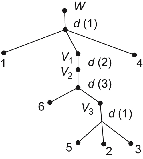
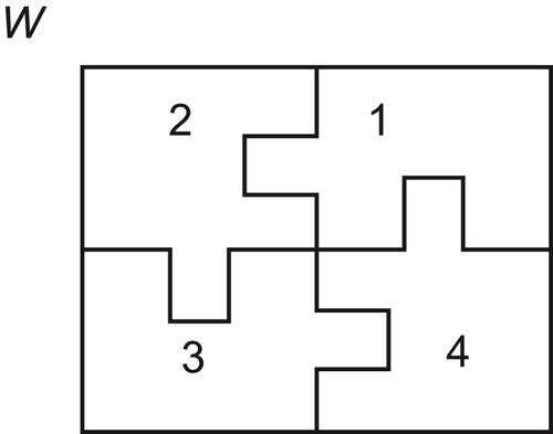
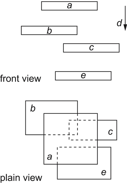
General automatic generation of assembly sequences is very complicated. Based on the hierarchical quotient space model, we present a monotonic planning algorithm. For a product, by compressed decomposition along some (disassembly) direction, the product is decomposed into sub-assemblies and parts. By successively compressed decomposition, the product is finally decomposed into a hierarchical tree structure. The assembly of the product simply goes on from bottom to top along the tree. Therefore, the computational complexity is reduced.
In automatic motion planning, i.e. collision-free paths planning in robotics, we present a topology-based model. In the model, the problem is first treated in some coarse topological space by ignoring the geometric details, after that we go deeply into the details of the physical space in some region that contains the potential solutions. Since the less-promising regions have been pruned off in the first step, the computational complexity can be reduced by the strategy. The estimation of the computational complexity and the applications of the method, such as multi-joint arm motion planning, are discussed.
Keywords
assembly sequences; characteristic network; compressed decomposition; configuration space; motion planning; rotation mapping graph (RMG); spatial planning; topological modelChapter Outline
5.1 Automatic Generation of Assembly Sequences
5.1.4 Computational Complexity
5.2 The Geometrical Methods of Motion Planning
5.2.1 Configuration Space Representation
5.2.2 Finding Collision-Free Paths
5.3 The Topological Model of Motion Planning
5.3.1 The Mathematical Model of Topology-Based Problem Solving
5.3.2 The Topologic Model of Collision-Free Paths Planning
5.4 Dimension Reduction Method
5.5.1 The Collision-Free Paths Planning for a Planar Rod
5.5.2 Motion Planning for a Multi-Joint Arm
5.1. Automatic Generation of Assembly Sequences
5.1.1. Introduction
5.1.2. Algorithms
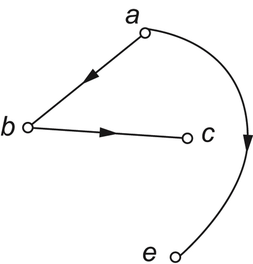
Directed Graph 
Definition 5.1
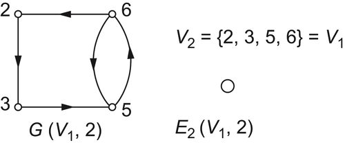
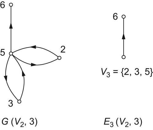
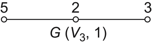
Compressed Decomposition
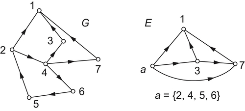
Cyclic Compressed Decomposition
Cyclic Compressed Decomposition Algorithm – Algorithm I
Assembly Planning Algorithm – Algorithm II
![]()
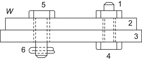
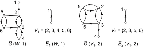
5.1.3. Examples
Example 5.1
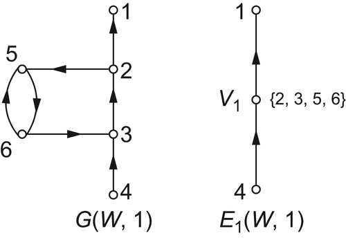
Example 5.2
5.1.4. Computational Complexity
The Completeness of Algorithms
Proof
Proposition 5.1
Proof
![]()
![]()
![]()
![]()
Corollary 5.1
Proposition 5.2
5.1.5. Conclusions