2.3. The Extraction of Information on Coarsely Granular Levels
Solving a problem in space  means investigating the attribute function of each element and the relationships among elements of X, i.e., the structure T, through analyzing and reasoning on domain X. If the multi-granular computing is adopted, the same attribute function f and structure T will be gained by analyzing and reasoning on a certain coarse granular world [X] of X. Thus, [f] and [T] in space
  must represent f and T to some extent, respectively. In Chapter 2, we have already discussed how [T] is induced from T when T is a topology or a semi-order. The construction of [f] will be discussed in this section.
Generally, constructing [f] from f is a domain-dependent problem. For example, when diagnosing an electronic instrument, our aim is to find the faulty element (or elements) of the instrument. The domain X is all electronic elements in the instrument. The attribute function f(x) is the functional parameters of each element in X. The aim of the diagnosis is to find which f(x) (or f(x)’s) is abnormal. In the case of the multi-granular diagnosis, the diagnosis first begins from a certain coarse granular level consisting of some components, for example,  {power-supply, amplifier, output-unit}. Thus, the attribute function [f] is represented by the functional parameters of these components, for example, the voltage of power supply, the amplification of amplifier, etc. How to choose these parameters in order to have more information regarding the fault of elements in X can be handled by an experienced troubleshooter easily. A knowledge-driven approach is generally adopted by many troubleshooters.
The construction of [f] still has some general principles. We next discuss these principles.
From the analysis of computational complexity above, we know that the relation between the goal estimation function and additional computation y is  , where the form of
  affects the computational complexity directly. If constructing a hierarchical structure (or [f]) such that
  , the complexity will be reduced to
  by the multi-granular computing. Conversely, if constructing a hierarchical structure (or [f]) such that
  , generally, only the polynomial complexity can be obtained by using multi-granular computing. At worst, if an improper structure (or [f]) is constructed, the computational complexity may not be reduced.
The preceding discussion implies that the multi-granular computing does not necessarily bring up high efficiency. The key is to construct a proper hierarchical structure. Generally, in multi-granular computing we follow the following principle. When a new problem space  is constructed from the original one
  , we expect to get from the former as more useful information regarding the latter as possible while keeping the new problem space simple.
Here, we propose a general principle for constructing quotient space. It is called ‘homomorphism principle’.
Homomorphism Principle
If there is a solution of problem p in space  , i.e., p is true, then a solution of corresponding problem [p] in
  also exists, i.e., [p] is also true. In other words, if there is no solution of [p] in
  , then there is no solution of p in
  either.
It seems that the homomorphism principle above is used extensively in our everyday life. Some examples are given below.
Example 2.7
Making an annual production plan, one first makes quarterly plans then monthly plans within each quarter and daily plans, etc., hierarchically.
Obviously, if there is an annual plan satisfying some given conditions, there exist quarterly plans, monthly plans and daily plans which satisfy the given conditions.
Conversely, if there is no quarterly plan, monthly plan or daily plan which satisfies the conditions, the annual plan cannot be worked out.
Example 2.8
In a find-path planning of an indoor robot, if the robot environment is rather complicated, it would be difficult to find a collision-free path at once by considering all the details of the whole environment. The path planning might have two levels. The first one, referred to as INTERROOM plan, is the planning of navigation from room to room without considering any details within the rooms. The second level, called INROOM plan, is the level of planning robot movements within the rooms.
It is obvious that if we cannot find a path from room to room, the entire path planning must fail.
We have seen that by the ‘homomorphism principle’, if we fail to find a solution in some parts of a coarse space, the corresponding parts of the original fine space have no solution either and can be pruned off. Clearly, through each granular level computing the search space is narrowed down. We now come to the key issue in our multi-granular computing. Whether the computational complexity can be reduced depends on how much search space is narrowed down through each granular level computing and how much additional computation is needed in order to have such a reduction. This is just the consideration that we need in constructing [f].
2.3.1. Examples
Before going deeply into the approaches to constructing [f], let us now examine some examples.
Example 2.9
In a national economy developing plan, if factories, mines and enterprises are elements of domain X, and  , x indicates the annual output value of these units. By hierarchical partition, some factories or enterprises compose a department A. The annual output value
  of each department A, certainly, is defined as
![]()
If  indicates the productivity of each factory, the productivity for A is defined as
![]()
Example 2.10
When throwing a ball upwards,  represents the attributes of the ball's motion at moment
  , where
  is the distance of the ball from the ground,
  is its velocity and
  is a time interval.
If we are only interested in the qualitative attributes of the motion, i.e., whether the ball goes upwards or downwards, or static, then time interval  is partitioned into five parts as follows.
 .
.
![]()
Let 
where,  , and
, and  denotes that the ball is on the ground,
  above the ground,
  goes upwards,
  goes downwards, and
  static. It is easy to have
![]()
Note that the range of function  is defined on some quotient set
  rather than
  . That is, partitioning Y into several equivalence classes and giving each equivalence class a symbolic name, the range of
  is just a set of these names. Sometime, it’s called a qualitative description of
  .
.
In summary, assume that  is known.
  represents some attribute of element
  . The point is how to choose the value of
  that can properly mirror the feature of the whole set A representing by the attribute
  and satisfies the homomorphism principle above. Generally,
  may be a value from Y or [Y].
More generally, given some local information of a set, we want to find the global information such that it can depict the features of the whole set. For example, the feature extraction of images in pattern recognition is somewhat similar to the above problem, where  (color, gray-level) is extracted from each pixel x, while
  represents the feature of regions or the whole image. We next present some common approaches to constructing function
  .
.
2.3.2. Constructing [f] Under Unstructured Domains
Starting from the domains X where elements are independent or near-independent of each other, we call it unstructured domains.
In terms of statistics, this amounts to ‘mutually independent’ assumption for random variables. In topological terminology, it is equivalent to ‘discrete topology.’ So unstructured is a special structure.
1.  is a space, where T is a discrete topology and
  ,
,  is an n-dimensional Euclidean space. Assume that R is an equivalence relation on X. The corresponding quotient space is
  .
.  is an attribute function on
  .
.
(1) Statistical method
Since X is unstructured,  depends on
  completely. From statistics, attribute
  of X can be regarded as a set of mutually independent random variables. Thus, attribute
  of [X] can be defined as some kind of statistics.
(2) Inclusion principle
If  , define
  as a specific point within
  where
where  is a convex closure of B. For example,
![]()
![]()
In Section 2.3.1, many examples for extracting  belong to the inclusion principle.
(3) Combination principle
If A is a finite set,  can be defined as follows
2.  is a set-valued function, i.e.,
  ,
,  is a subset of Y.
(1) Intersection or union method
![]()
If Y is a complete semi-order lattice, then  and
and  or
or  and
and  are equivalent. The method is equal to the inclusion principle in 1.
An example is given below.
Assume that A={a set of quadrilaterals on a plane}=
a1={a set of squares}, a2={a set of rectangles},
a3={a set of diamonds}, a4={a set of parallel quadrilaterals},…
Let
Now, we can use  to define
  , for example,
  .
.
(2) Quotient space method
Thus,  represents the image of
  on
on  via natural projection p. The range of
  is
is  .
.
In qualitative analysis,  is partitioned into
  and
and  simply,
  denotes as ‘0’ and
  as ‘+’, respectively. R is partitioned into
  , and
, and  , simply,
  as ‘0’,
  as ‘–’, and
  as ‘+’, respectively. Defining
  , we then have the same results as shown in Example 2.10 of Section 2.3.1. Using the elements (or subsets) in quotient space [Y] to describe [f] is a useful method in qualitative reasoning especially. We’ll discuss the problem in Chapter 4.
2.3.3. Constructing [f] Under Structured Domains
Under the structured domains, the values of  that correspond to different element x are interdependent and are related to structure T. So from structure T, we can have some knowledge about
  . Generally, structure T may be classified into three main classes below.
(1) T is a topologic structure. For example, X is an n-dimensional Euclidean space. Then the Euclidean distance is its topologic structure T. Generally speaking, any metric space is an instantiation of topologic structures.
(2) Defining a semi-order relation on X, we have a semi-order structure T. Anyway, we can introduce a corresponding semi-order to any system which can be represented by a directed acyclic graph. Hence, semi-order relation represents a wide range of structures in real world.
(3) The structure of X can be induced by some operations defined on X. For example, given a unary operator  , i.e.,
  , it implies that a relation between elements x and
  is established. Linking these two elements by a directed edge, we define a directed graph corresponding to operator p. And, the directed graph determines a corresponding pseudo semi-order relation as well. If p is a multivariate operator on X,
  , it can also be represented by a graph. For example, each
  connects to y with a directed edge. And the n directed edges connected to y are linked by a curved arc. Then, we have a graph corresponding to p and it is somewhat similar to an AND/OR graph or a hyper-graph. From the graph, we can define its structure, T. So the relation among elements can be defined by multivariate operation p as well.
This section only tackles the problem of constructing [f] under topologic structures. For semi-order structures, see discussion in Chapter 3.
Assume that  and
and  are two topologic spaces.
  is an attribute function on X. The continuity of f is a key issue in analyzing the properties of
  . For example, we are given a premise
  , in order to affirm if the conclusion
  holds or not, our objective is to determine if there exists a sequence
  of reasoning steps from
  to
to  . If so, the conclusion
  holds, otherwise,
  does not hold. This is similar to the concept of ‘path-connected’ in topology. We show the concept as follows. If
  , there exist
  such that each line segment
  belongs to A, then
  and
and  are said to be path-connected in A. Therefore, by introducing a proper topology T into X, the problem that if
  can infer
  is transformed to that of whether
  and
and  belong to the same path-connected component. In Section 2.5, we’ll discuss the problem in more details.
Generally, X is rather complicated. It is not easy to judge whether any two given points belong to the same path-connected component. By using transformation function  , the problem can be transferred into an easier one if the structure of Y is simpler than X. Obviously; we expect that if set
  is a connected, the transformed set
  is still connected. From topology, we know that if
  is a connected set, the image
  of A is also a connected set in Y when f is continuous. Once again it shows that the continuity of function f is a very significant property.
By partitioning  we have a quotient space
  . From f we induce a function
  on [X]. Obviously, we expect that [f] would still be continuous. Unfortunately, it is not true generally. Even so we expect that [f] still remains some weaker continuity than the strict one in favor of the analysis.
1. Constructing 
First, we introduce some concepts below.
Definition 2.5
Assume that  is a metric space. Let
  ,
,  .
.
Definition 2.6
R is an equivalence relation on  . Let
. Let  , where [X] is a quotient space corresponding to R.
  is said to be fineness of R. Intuitively,
  can be regarded as ‘the maximal diameter’ of equivalence classes corresponding to R.
Definition 2.7
Assume that  , R is an equivalence relation on
  , and [X] is a quotient space under R. Let
  .
.  is said to be fineness of R with respect to f.
Definition 2.8
Assume that  . Let
. Let  . M is called the ratio of expansion and contraction of f, or simply REC.
Definition 2.9
Assume that  , where
  is a metric space. Given a positive constant
  , if
, if  there exists an open set u(x) such that
  . f is said to be
  -continuous on X, where
  .
.
Proposition 2.10
Assume that  is a continuous function, [X] is a quotient space of X. Define
  as
as  , where
  .
.
Suppose that M is a REC of f and the fineness of [X] is l. Given  , we obtain that
  is a
is a  -continuous function on X, where
  is a natural projection function.
Proof:
Since the fineness of [X] is l, we can write the diameter of 
 .
.
From the REC M of f, we have the diameter of 

From the definition of [f], we obtain
![]()
That is
![]()
Given  by letting
  be small enough such that
  , we have that
  is
is  -continuous at x.
  is
is  -continuous on X.
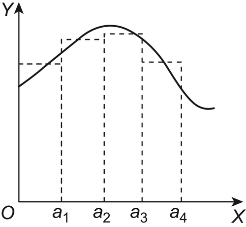
Example 2.11
As shown in Fig. 2.1,  is a continuous function.
Assume that  . Axis X is partitioned into several intervals equally, each interval
  with length
 . If using a step function as follows
Proposition 2.10 indicates that under quotient space transformation the continuity of the transformed function does not always hold but α-continuity, a weak continuity, is preserved. It implies that if viewing from a coarse granular level, the properties of the original function become rough (fuzzy). Intuitively, it may be likened to copperplate etching technique. The coarser the etching grain-size of a copper plate the rougher its image.
Generally speaking, instead of some attribute f in the original space, a new attribute  can be used for describing the corresponding one in its quotient space. In order to transform the original attribute function f into
  , it is needed to redefine the function. As we know, the original function f(x) is defined on ‘all neighborhoods of x’ or ‘a neighborhood existed in x’, we now need to redefine
  -f(x) on ‘a fixed
  -neighborhood of x’ or ‘some fixed neighborhood of x’. This idea has also been used in the mathematical morphology method of pattern recognition (Serra, 1982).
We might as well try to analyze two basic operations in mathematical morphology from our granular computing point of view.
Definition 2.10
Assume that X is a domain.  ,
,  , a corresponding subset
  is given on X.
  is called a structural element with respect to x. Define
![]()
Dilation and erosion are two basic operations in mathematical morphology. Any morphological transformation can be obtained through union, intersection and deference of these two operations.
In topology, the minimal closed set containing A is called a closure of A denoted by  and is defined as:
 is an open set containing x.
![]()
Accordingly, given a set A, the maximal open set being contained by A is called an inner-kernel of A and denoted by  . Mathematically, the definition is as follows:
![]()
Either closure or inner-kernel operation can be used for defining a topologic structure of a space. Hence, closure and inner-kernel operations are two basic operations in topology.
It is clear that both  and D(A) are quite similar. So long as replacing ‘
 ’ (in the definition) by a fixed subset B(x), the concept
  becomes D(A). So the concept D(A) is equivalent to ‘α-closure’. The same is true for the relation between
  and E(A). Thus, E(A) is equivalent to ‘α-inner kernel’.
We know that D(A) and E(A) are the rough descriptions of closure  and inner-kernel
  in the coarse granular level, respectively. The aim of mathematical morphology is to extract some essential characteristics of images while ignoring their details. This is identical with the ‘α-∗∗’ concept. As J. Serra pointed out ‘The images under study exhibit too much information and the goal of any morphological treatment is to manage the loss of information through the successive transformations’ (Serra, 1982). The multi-granular computing is similar to the above idea.
The concept of ‘α-∗∗’ is an outcome of hierarchy. The similarity between the concept of ‘α-∗∗’ and the concept of dilation (or erosion) in mathematic morphology indicates that our quotient structure model can be extended to more general cases.
When space X is transformed to its quotient space [X], i.e.,  , where p is a natural projection, the attribute ‘∗∗’ becomes ‘α-∗∗’. Similarly, when
  , where
  is a subset of X, the
  (or
(or  ) becomes D(A) (or E(A)). In this case, if X is an original space,
  can be regarded as a ‘quotient space’ of X by considering each
  as an element.
Definition 2.11
Assume that  is a metric space. If X cannot be represented by the union of two non-empty sets A and B that satisfy the following condition (2.9)
![]() (2.9)
(2.9)
![]()
Property 2.1
Assume that  , R is an equivalence relation on X, and
  . The ratio of expansion and contraction (or REC) of f is M. We have:
![]()
Proof:
From the definitions of  and
and  , we have the proof directly.
Theorem 2.1
Assume that  is continuous, X is connected, R is an equivalence relation on X, and
  . The REC of f is M. Define
![]()
That is, we take on  at any point
  as the value of
  at point
  . Thus,
  is 2Ml-connected.
Proof:
Let  . From Property 2.1, we have
  .
.
Reduction to absurdity, assume that  is not d-connected. Letting
  , there exist non-empty sets A and B that satisfy (Fig. 2.2):
![]()
We first show that
![]()
Since
![]()
![]()
That is,
![]()
Similarly
![]()
Since  and
and  , by letting
  , again from
  and
and  , we have
  .
.
Similarly, we have  .
.
From  .
.  and
and  are closed sets and f is continuous, we know that
  and
and  are closed on X. Therefore,
  , where
  and
and  are non-empty closed sets and
  . Thus, X is not connected, which contradicts the assumption that X is connected.
Consequently,  is d-connected.
The concept of d-connected can be regarded as a description of the degree of connectivity of a set. The smaller the d, the closer to true connectivity the d-connectivity is. In other words, regarding any two sets on X as being connected provided their distance is less than d, then we have d-connected. The theorem indicates that if the REC of f is fixed, the roughness of connectivity of images in the coarse granular level is inversely proportional to the fineness of R. That is, the finer the partition, the less rough (finer) the connectivity of images in the coarse granular level. Conversely, keeping the fineness of R fixed, the roughness of connectivity is proportional to the REC of f. That is, the larger the REC the rougher the connectivity of the mapped images. The above intuition can accurately be proved by our quotient space model.
Obviously, the concept of d-connectivity is an instantiation of the concept of ‘ ∗∗’ that we mentioned before. After the partition, some information must be lost in coarse granular levels. Generally, it is hard to preserve the original attributes (e.g., continuity, connectivity, etc.) of the original space. By introducing the concept of ‘
 ∗∗’ attributes, weaken attributes, the original attributes will remain valid in a relaxed sense. This will provide a useful clue to the analysis of coarse granular levels.
For some concept such as connectivity in topology, a set either is connected or not. Either of the two facts must be true. By introducing ‘d-connectivity’, the different degrees of connectivity can be described. This is just like the concept of membership functions in fuzzy mathematics. The concept of ‘ ∗∗’ attributes that we presented here virtually relates our methodology to that of fuzzy mathematics. It makes granular computing more powerful.
2. Constructing 
In the preceding section, we know that the value of  can also be represented in quotient space
  of Y. We next present its properties.
Assume that  and
and  are topologic spaces,
  is a one-to-one corresponding function, R is an equivalence relation on X. [X] is a quotient space of X with respect to R.
Definition 2.12
Define an equivalence relation  on Y such that:
![]()
That is, x and y are equivalent on Y if and only if the original images of x and y are equivalent on X.  is said to be an equivalence relation on Y induced from R via f or an induced equivalence relation from R.
Conversely, if  is an equivalence relation on Y, define an equivalence relation on X such that
 via f or an induced equivalence relation from
  , where f is not necessarily one-to-one correspondent.
![]()
Lemma 2.1
Assume that  and
and  are topologic spaces,
  , R is an equivalence relation on X,
  is an equivalence relation on Y induced from R. Let
  and
and  be quotient spaces corresponding to R and
  , respectively. Define
 and
and  are natural projections. Then, for
  , we have
  .
.
![]()
Proof:
Obviously,  .
.
Conversely, is a set composed by elements of [X], where the element of [X] is a subset of X.
Theorem 2.2
Assume that  and
and  are topologic spaces, R is an equivalence relation on X,
  is an equivalence relation on Y induced from R,
  and
and  are quotient spaces with respect to R and
  , respectively,
  is a continuous function. Let
  be
be  , where
  and
and  are projection functions. Thus,
  is continuous.
Proof:
For  , assume that
  is an arbitrary neighborhood of
  . Let
. Let  . Regarding
  as a set of Y, it is open. Since f is continuous, we know that u is an open set on X. From Lemma 2.1, we can see that u is a set on [X]. Thus, together with the definition of quotient topology, it implies that u is a neighborhood of a. From the definition
  , we have that
  is continuous at a. That is,
  is continuous.
Corollary 2.1
If  is an equivalence relation on Y and R is an equivalence relation on X induced from
  .
.  is continuous. Then
  , for
, for  is continuous.
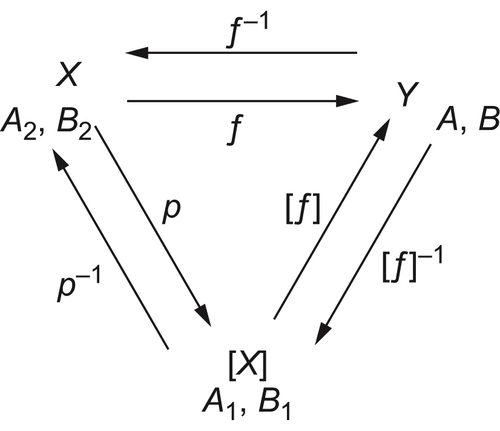
Theorem 2.2 presents another approach for constructing function [f]. It has a wide-ranging application, for example, qualitative reasoning in Al. We next analyze the Example 2.11 in Section 2.3.1.
When an object is thrown upwards, its state at moment x can be represented by  , where
  and
and  indicate its distance from the ground and velocity at moment x, respectively. Now only the qualitative properties of its state are paid attention to. The range
  of
of  is partitioned into two classes {0} and
  . While the range
  of
of  is divided into three classes {0},
  , and
, and  .
.  is regarded as a continuous function on
  . The preceding partition corresponds to an equivalence relation
  on Y. From Theorem 2.2, in order to construct [f], we need an equivalence relation on X induced from
  .
.
R is partitioned into  , {0} and
  ,
,  is its induced equivalence relation on X. Then,
 indicates the inverse transformation of the first component of f,
![]()
The combination equivalence relation of  and
and  is
is  and
and
![]()
Let  and
and  be quotient spaces with respect to
  and
and  , respectively. From Theorem 2.2, we know that
  , where
  is a projection function, and [f] is a continuous function of
  .
.
If the first component {0},  of [Y] is named as ‘0’, ‘+’; the second component
  and
and  of [Y] as ‘–’, ‘0’ and ‘+’, we have [f]((t1, t2)) = (+, −), [f]({t1}) = (+, 0), etc. These results are consistent with that shown in Example 2.11 of Section 2.3.1.
From our quotient space model, a strong property of [f] is discovered, that is, [f] is a  continuous function, if it is constructed in the way that we already showed. In the light of the result, we can see that this is one of the possible ways for partitioning X (or Y).
2.3.4. Conclusions
In this section, we have discussed how to establish a function [f] on [X] induced from f. When X is an unstructured domain, we presented four basic methods for constructing [f], that is, statistics, closure, quotient space and combination methods. If X is a structured domain, only topologic structures and continuous function f are involved. When [f] is a  function, we introduced the concepts of
  continuity and
  connectivity and established the corresponding properties of [f]. When [f] is a
  function, we presented an approach for constructing function [f] which guarantees its continuity.
So far we have established all three elements of problem space  . Further discussion will be presented in Chapters 3 and 4.
..................Content has been hidden....................
You can't read the all page of ebook, please click here login for view all page.