5.2. The Geometrical Methods of Motion Planning
The problem addressed here is a specific motion planning problem, known as the findpath problem in robotics. The problem is stated as follows: Given the descriptions of an object and a collection of obstacles in a 2- or 3-dimensional space, given also the initial and desired final configurations for the object, to find a collision-free path that moves the object to its goal, or determine that no possible path exists.
The common theme in motion planning work is the idea of representing the problem in such a way that the object to be moved is a point, and the point is moved through a configuration space that may not necessarily be equal to the 2-or 3-dimensional space of the physical problem. It is called configuration space representation, or  for short (Lozano-Perez, 1973; Lozano-Perez and Wesley, 1979; Brooks and Lozano-Perez, 1982; Brooks, 1983).
5.2.1. Configuration Space Representation
A Planar Moving Object Without Rotation
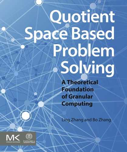
As shown in Fig. 5.12, A is a convex polygonal moving object and B is a convex polygonal obstacle. Assume that A is a rigid object moving among obstacles without rotation.
We associate a local coordinate frame with A. The configuration of A can be specified by the x, y position of the origin a of the local coordinate frame, and a θ value indicating the rotation of the local frame relative to the global one. The space of all possible configurations of A is its configuration space. A point in the space represents a particular position of a, the reference point of A, and an orientation of A.
Due to the presence of obstacles some regions of the configuration space are not reachable. These regions are called configuration obstacles, illegal or forbidden regions. Therefore, the moving object is shrunk to a point in the configuration space, and the obstacles are expanded to form configuration obstacles (see Fig. 5.12 shaded area). The formal definition of configuration obstacle is given below.
Definition 5.2
The configuration space of moving object A is denoted by  . Symbol
  represents the configuration obstacle of B in
  . We have
 indicates the moving object A with configuration x.
![]() (5.1)
(5.1)
Obviously, if  then collides with B. Otherwise,
  , does not intersect B.
Definition 5.3
Let  be the interior points of B in . Thus,
![]() (5.2)
(5.2)
Obviously,  .
.
Therefore, ‘findpath’ problem can be stated as to find a sequence of configurations of A such that they are inside of  but outside of
  , where
  are obstacles and R is the whole physical space (see Fig. 5.12).
The key issue of path planning is to construct configuration obstacles.
5.2.2. Finding Collision-Free Paths
Once configuration obstacles or their approximations have been constructed, there are several strategies for finding a path outside the configuration obstacles for a moving point that represents object A.
Visibility Graph
If all obstacles  are polygons and A is also a polygon with a fixed orientation, then
  obstacles with parameter
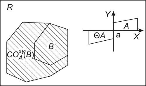
  are polygons as well. The shortest safety path of A consists of a set of line segments which connect the starting point, some vertices of polygon and the goal point, as shown in Fig. 5.13. It is called the visibility graph method or
  method.
The algorithm can be extended to 3-dimensional spaces. If  is known, the safety path can be found as the 2-dimensional case. But the path being found is not necessarily optimal. Sometimes, no safety path can be found even if it does have a collision-free path.
When A is a 3-dimensional object with rotation,  is a complex curved object in a 6-dimensional space, the method cannot be used directly. Some approximations may be adopted such as the slice projection approach, etc.
Subdivision Algorithm
The fundamental process of the subdivision algorithm (Brooks and Lozano-Perez, 1982) is that configuration space is first decomposed into rectangles with edges parallel to the axes of the space, then each rectangle is labeled as E (empty) if the interior of the rectangle nowhere intersects obstacles, F (full) if the interior of the rectangle everywhere intersects obstacles, or M (mixed) if there are interior points inside and outside of obstacles. A free path is found by finding a connected set of empty rectangles that include the initial and goal configurations. If such an empty cell path cannot be found in the initial subdivision of , then a path that includes mixed cells in found. Mixed cells on the path are subdivided, by cutting them with a single plane normal to a coordinate axis, and each resulting cell is appropriately labeled as empty, full, or mixed. A new round of searching for an empty-cell path is initiated, and so on iteratively until success is achieved. If at any time no path can be found through non-full cells of greater than some preset minimal size, then the problem is regarded as insoluble.
Other Methods
There are several known geometric approaches for finding collision-free paths such as the generalized cone method (Brooks, 1983), the generalized Voronoi graph method, etc. We will not discuss the details here.
..................Content has been hidden....................
You can't read the all page of ebook, please click here login for view all page.