4.3. Reasoning (Inference) Networks (1)
A great number of reasoning processes can be represented by a graph search.
First, let see an example.
Example 4.1
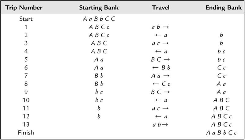
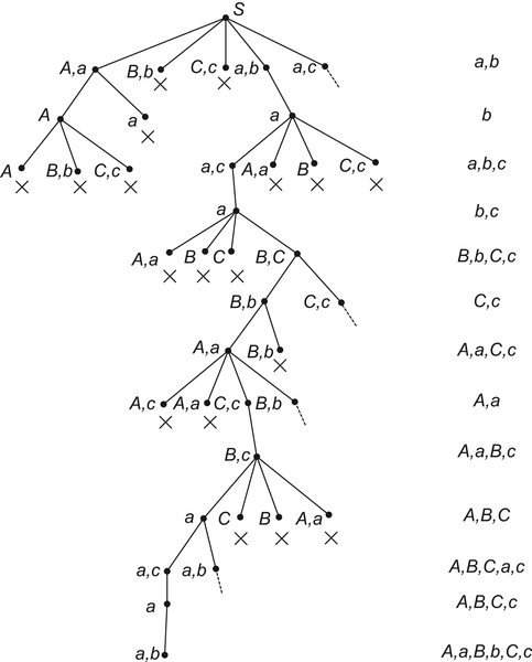
The jealous husbands problem is one of the well-known river-crossing puzzles. Three married couples denoted by {A a, B b, C c} must cross a river using a boat which can hold at most two people and subject to the constraints: (1) no woman can be in the presence of another man unless her husband is also present, (2) only three men {A,B,C} and one woman {a} master rowing technology. Under the constraints, we have two heuristic rules: (1) there cannot be both women and men present on a bank with women outnumbering men, since if there were, some woman would be husbandless, (2) only the following ways of river crossing exist: one or two men, woman a or with any other woman, or any couple. Where the married couples are represented by A (male) and a (female), B (male) and b (female), and C (male) and c (female), respectively.
Using the heuristics, we have a shortest solution to the problem shown in Table 4.1. There are 13 one-way trips. The river-crossing process can be represented by a graph as shown in Fig. 4.1.
That is, given a directed graph G, a premise A and a goal p in G, a reasoning process can be regarded as finding a path from A to p in the graph. Since a directed acyclic graph can be represented by a semi-order space  , the reasoning mechanism can then be depicted as follows.
(1)  is a premise, Let
  and a goal
(2) Reasoning rule: if b is a direct successor of a, then  .
.
If we find a p in  such that
  , then p holds. Otherwise, p does not hold.
In order to change the certain reasoning model above into an uncertain reasoning model, the following two problems must be solved: (l) the representation of the uncertain premise; (2) the representation of the uncertain reasoning rule. As mentioned before, uncertain information can be described in different grain-size spaces, while uncertain reasoning rules can be represented by probability. We have the following uncertain reasoning model:
(1) For  , we define a function
  on A
on A
(2) D is a set of edges on a reasoning network. Define a reasoning function 
(3) Reasoning rule: if b is a direct successor of a, for  , define an reasoning rule
F is an arbitrary combination function, for example, 
(4) Given a goal  , by the model we have
  , then p holds with confidence d.
Table 4.1
River-Crossing Process
| Trip Number | Starting Bank | Travel | Ending Bank |
| Start | A a B b C C | ||
| 1 | A B C c | a b → | |
| 2 | A B C c | ← a | b |
| 3 | A B C | a c → | b |
| 4 | A B C | ← a | b c |
| 5 | A a | B C → | b c |
| 6 | A a | ← B b | C c |
| 7 | B b | A a → | C c |
| 8 | B b | ← C c | A a |
| 9 | b c | B C → | A a |
| 10 | b c | ← a | A B C |
| 11 | b | a c → | A B C |
| 12 | b | ← a | A B C c |
| 13 | a b→ | A B C c | |
| Finish | A a B b C c |
Especially, when d = 1, p holds. Otherwise, if d = 0, p does not hold.
Meantime, another two problems must be solved in order that reasoning can be made in a multi-granular world. First, given an uncertain reasoning model on X and its quotient space [X], how to construct a corresponding reasoning model in [X]? This is a projection problem. How to obtain some useful information on X from the reasoning that we draw on [X], this is the problem about the relation between two reasoning models. Second, given two reasoning models on quotient sets  and
and  , how to get a whole understanding about X? This is the synthesis problem of different evidences. We first discuss the projection problem.
4.3.1. Projection
An uncertain reasoning model is represented by is a reasoning function defined on A. T is a semi-order structure. F:
  is a function called a reasoning rule.
![]()
In essence, so-called reasoning is to answer whether p can be inferred from A, or to what degree of confidence p does hold, when given domain structure T and reasoning rule F.
Projection problem is that given reasoning model with respect to X and its quotient set X1, find the corresponding reasoning model on X1.
Since X1 is a quotient set of X, Edges  on X1 is the corresponding quotient set of D. First, we define
![]()
Let  be a set of all equivalence classes
  defined above. At present
  is not a partition of D. Let E0 be a set of edges of D not belonging to any equivalence class in
  . Adding E0 into
  , we have D1. D1 is a quotient set of D.
  is undefined in E0.
A1 is a quotient set with respect to A. p1 is the equivalence class corresponding to p, and  .
.
R is an equivalence relation with respect to X1.  on
on  is an induced quotient quasi-semi order from R. If R and T are compatible, then
  is a quotient semi-order on X1.
Again, the methods for constructing f1 and g1 are given below. For example, by using ‘combination principle’, we define .
.
![]()
![]()
Taking the same F as the reasoning rule, we have a reasoning model of X1 as
![]()
Example 4.2
Assume that
![]() (4.1)
(4.1)
![]()
![]() (4.2)
(4.2)
We have the following proposition.
Proposition 4.1
Proof
Assume that in X from  and via
  , we infer p and
  .
.
According to the reasoning steps, by induction, when  , the conclusion obviously holds. Now assuming that for n < m, the conclusion holds, we show that for n = m the conclusion still holds.
Assume that  . From the assumption, we have
  .
.
(1) If  , since
  , we have
 , we have
  . Namely
![]()
![]()
(2) If  , assuming that
  , since
  , we have
  . From the above definition, we have
![]()
![]()
![]()
The proposition indicates that the projection defined above satisfies the ‘homomorphism principle’. That is, if in the high (coarse) abstraction level, we infer that p1 holds with confidence <d, then in the low (fine) level, the corresponding p holds with confidence <d as well.
Simply speaking, if there is no solution in some regions of high abstraction level, i.e., p1 holds with low confidence, then, there isn’t any solution in the corresponding regions of any lower level. This means that based on the result that we infer from high abstraction levels, the possible solution regions in low levels are narrowed. This is the key for reducing computational complexity by hierarchical problem-solving strategy, as discussed in Chapter 2.
When equivalence relation R corresponding to X1 is incompatible with the semi-order structure T of X, we must revise R such that it is compatible with T, as we have discussed in Chapter 1.
4.3.2. Synthesis
In our reasoning model, uncertain information is represented at different grain-size worlds. The information observed from different perspectives and aspects will have different forms of uncertainty. We will consider how to synthesize the information with different uncertainties.
Assume that X1 and X2 are two quotient sets of X. Two reasoning models  and
and  on X1 and X2 are given. The synthesis of reasoning is to find a new reasoning model
  in the synthetic space X3 of X1 and X2.
According to the approach indicated in Chapter 3, we have
(1) X3: the least upper bound of spaces  and
and 
(2) D3: the least upper bound of spaces  and
and 
(3)  : the least upper bound of semi-order structures
  and
and  .
.
In fact, when X3 and  are fixed, D3 is uniquely defined. Therefore, X3 is defined first, then
  and finally D3 is obtained from
  .
.
After the projection operation of attribute functions on X has been decided, the synthetic functions  and
and  are known based on the synthetic method shown in Section 3.6. Let
![]()
![]()
If the same reasoning rule F is used, we have a reasoning model in the synthetic space X3 as follows.
![]()
We next use our synthetic approach to analyze Dempster-Shafer combination rule (or D-S combination rule) in Belief Theory.
Example 4.3
First, we introduce briefly some basic concepts in Belief Theory (Shafer, 1976).
Assume that X is a finite domain,  is a power set of X. Define a function
  such that
(1) 
(2) 
m is called a basic probability assignment on X. Let  . Bel(A) is said to be a belief function.
Since belief function (Bel) is defined on P(X), when P(X) is regarded as a new set X1, then Bel is just a function on X1. Therefore, Bel is an attribute function on P(X).
Assume that m1 and m2 are two given attribute functions on X1 and X2, respectively. We have two problem spaces  and
and  , where
  is a topology on
  , i = 1, 2.
The synthesis of the two spaces is as follows.
Let X3 be the least upper bound of spaces X1 and X2, T3 be the least upper bound of topologies T1 and T2.
Define a projection operation of attribute functions as follows.
Assume that m3 is an attribute function on X3.
Letting  :
: be a nature projection, we have
  . That is,
![]() (4.3)
(4.3)
As mentioned in Section 3.6, the synthesis of quotient spaces  and
and  is equivalent to that m3 satisfies Formula (4.3). But the solution of m3 is not unique. Some optimal criterion must be introduced.
It’s known that the attribute function in the coarse level, except itself, cannot provide more information to the attribute function in the fine level. In other words, besides that m3 satisfies (4.3), it must preserve a maximal uncertainty, or in terms of information theory, ‘a maximal entropy’.
When X is a finite set, the entropy of  can be defined as
![]() (4.4)
(4.4)
The maximal criterion is
![]() (4.5)
(4.5)
When X is a finite set, the two quotient spaces of X are
![]()
The least upper bound space X3 of X1 and X2 is
![]()
We first assume that all  . Let
. Let
![]()
From (4.3), we have
 (4.6)
(4.6)
From (4.4), we can write
![]() (4.7)
(4.7)
Using Lagrange multiplier, we have
![]()
Finding the partial derivative of the formula above with respect to each  , and letting its result be zero, we have a set of equations
![]() (4.8)
(4.8)
Again from (4.6), we can write
 (4.10)
Since m1 and m2 are basic probability assignments in  and
and  , we have
![]()
Letting  , we obtain
  ,
,  and t-s=0.
Letting t=s=1, we have
![]()
Finally,  .
.
This is just the D-S combination rule, where  ,
,  and
and  are basic probability assignments. The combination rule that we obtained is from the maximal entropy principle.
In case of some of  being empty, we will discuss this next.
Example 4.4
![]()
![]()
Since  ,
,  ,
,  and
and  , we have
![]()
Since  ,
,  .
.
That is,  . But from
  , we have
  . This is a contradiction. Therefore, there does not exist such a
  that satisfies Formula (4.6).
As discussed in Section 3.6, when the  satisfying Formula (4.6) does not exist, similar to the least-squares, a criterion can be introduced. Combining with the given criterion, an optimal solution can be obtained.
When some of  are empty,
  is defined as follows.
Let
![]()
![]()
![]()
Formula (4.6) becomes
 (4.11)
Formula (4.11) may not have a solution, so a weighted least-squares function is used as shown below. and
and  are weights (constants).
As an optimal criterion, ‘the maximal entropy principle’ is still used. That is,
![]()
Let
![]() (4.12)
(4.12)
Find a  such that the right hand side of Formula (4.12) is minimum.
By using the Lagrange multiplier, we have
![]() (4.14)
(4.14)
Finding the partial derivative of Formula (4.14) with respect to each  and letting the result be zero, we have a set of equations.
 is only over all j in
  , the second sum
  is only over all i in
  .
.
![]() (4.15)
(4.15)
Since  , we have
  , i.e.,
  .
.
Finally, we have is over all
  .
.
 (4.18)
Formula (4.18) is just the D-S combination rule.
We therefore conclude that, the D-S combination rule can be inferred from the synthetic method of quotient spaces by using ‘maximal entropy principle’. It is noted that D-S rule is simple and is easy to be used, but weights  and
and  shown in Formula (4.17) are artificial. It means that we might choose some other optimal criteria such that different combination rules would be obtained to aim at different issues.
Domain structural knowledge, the relationships among elements, for example, the age order among people, the Euclidean metric relations in a two-dimensional image, etc., is not considered either in membership function or in belief function. But it is quite important in multi-granular computing. In our model, taking all factors, including domain, structure and attribute, into consideration and when being transformed from one grained world to the others, their structures are required to satisfy the homomorphism principle. By the principle, it’s known that if a proposition is rejected in a coarse-grained world, it must be false in the fine-grained world. Therefore, due to the principle we can benefit from multi-granular computing.
4.3.3. Experimental Results
In this section, we will show the advantage of multi-level graph search (or reasoning) based on quotient space theory by data validation (He, 2011).
The experimental setting is searching the shortest path on three different kinds of networks, i.e., random, small-world and scale-free networks that randomly generated from data. The numbers of their nodes are 100, 200, 300, 400 and 500, respectively. The experiments are implemented on a Pentium 4 computer (main frequency 3.00 GHz, memory capacity 2 GB) using Windows XP SP3. Our method is multi-level (generally, 5–6 levels) search based on quotient space theory. Dijkstra and Floyd algorithms are well-known search algorithms (see Dijkstra, 1959; Floyd, 1962, for more details).
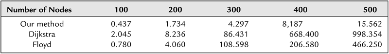
From the results (Tables 4.2–4.4), it’s shown that two orders of magnitudes of CPU time can be saved by multi-level search when the scale of networks becomes larger. But the performances slightly reduce, i.e., the ratio between the optimal path found and the real shortest path is 85% in the multi-level search.
Table 4.2
Total CPU Time (in seconds) in Random Networks
| Number of Nodes | 100 | 200 | 300 | 400 | 500 |
| Our method | 0.939 | 1.356 | 3.112 | 6.634 | 12.171 |
| Dijkstra | 1.719 | 9.797 | 91.141 | 565.391 | 1002.125 |
| Floyd | 0.940 | 4.220 | 118.630 | 212.030 | 511.560 |
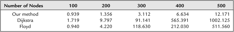
Table 4.3
Total CPU Time (in seconds) in Small-World Networks
| Number of Nodes | 100 | 200 | 300 | 400 | 500 |
| Our method | 0.640 | 2.403 | 6.659 | 14.330 | 22.262 |
| Dijkstra | 2.758 | 10.546 | 87.239 | 700.540 | 1100.200 |
| Floyd | 0.790 | 4.783 | 132.743 | 230.412 | 498.317 |
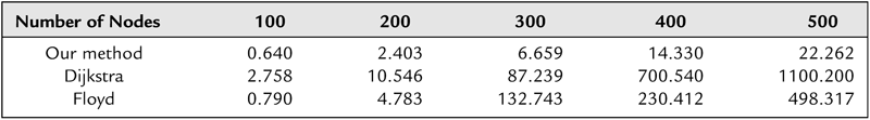
Table 4.4
Total CPU Time (in seconds) in Scale-Free Networks
| Number of Nodes | 100 | 200 | 300 | 400 | 500 |
| Our method | 0.437 | 1.734 | 4.297 | 8,187 | 15.562 |
| Dijkstra | 2.045 | 8.236 | 86.431 | 668.400 | 998.354 |
| Floyd | 0.780 | 4.060 | 108.598 | 206.580 | 466.250 |
..................Content has been hidden....................
You can't read the all page of ebook, please click here login for view all page.