5.3. The Topological Model of Motion Planning
The idea of representing the motion planning problem in configuration space is to transform the moving object into a point and have the point move through that space. Generally, this is simpler than to consider the original object moving through the physical space, although the dimensions of the configuration space are usually higher than those of the physical one. The drawback of the above geometric approaches is in need of considering all geometric details throughout the entire planning process. When the environment is rather complicated, the computational complexity will increase rapidly.
From the multi-granular computing strategy, the problem can be solved in such a way that the problem is treated in some coarse-grained space by ignoring the geometric details first, after that we go deeply into the details of the physical space in some regions that contain the potential solutions. Since the less-promising regions have been pruned off in the first step, the computational complexity can be reduced by the strategy.
If the motion planning problem can be represented by a topological model, and under certain conditions the geometric details can be omitted, then we may deal with the problem in the simplified topologic space. Thus, we discuss the topological model first (Zhang and Zhang, 1982a, 1982b, 1988a, 1988b, 1988c, 1988d, 1988e, 1990c; Schwatz and Shatic, 1983a, 1983b; Chien et al., 1984; Toussaint, 1985).
5.3.1. The Mathematical Model of Topology-Based Problem Solving
Some problem solving can be stated as follows. From a given starting state, by a finite number of operations, then the final goal is reached. This is similar to the concept of arcwise connectivity in topology.
Arcwise Connected Set
The Topologic Model of Problem Solving
X is a domain. Introducing a topology T into X, then we have a topologic space  . Assume that
  is a set of mappings. If
  is a mapping, p is called an operator on X. Assume that P satisfies the following conditions.
Definition 5.4
Assume that P is a set of operations on X. If for  and
and  , x and
  belong to the same arcwise connected component on , P and T are called consistent. If
  and
and  belong to the same arcwise connected set, there exists
  , then P is called complete.
In a general topologic space, the arcwise connectivity can be defined as follows.
Since the combination of an operation is still an operation, the implement of a finite number of operations is equivalent to that of one operation. So the problem solving can be restated as follows.
Starting state  , goal state
  and a set P of operations are given. The aim of problem solving is to find if there is an operation
  such that
  . If such an operation exists, it’s said that the corresponding problem has a solution; otherwise, there is no solution. If the solution exists, the goal is to find the corresponding operator p.
Proposition 5.3
Assume that a set P of operations and topology T on are consistent and complete. and are starting and goal states, respectively. The corresponding problem has a solution  and belong to the same arcwise connected component on X.
Proof
The proposition shows that a problem solving can be transformed into the arcwise connectivity judgment problem in a topologic space.
We introduce some properties of connectivity below.
Primary Properties of Connectivity
Property 5.1
If A is arcwise connected, then A is connected.
Property 5.2
Assume that  is a continuous mapping.
  and
and  are topologic spaces. If X is connected, then
  is connected on Y.
Property 5.2 shows that the continuous image of a connected set is still connected.
Property 5.3
Property 5.4
If A is connected and  , then B is connected, where
  is the closure of A.
Definition 5.6
Property 5.5
If  is connected and locally arcwise connected, then X is arcwise connected.
Property 5.6
Properties 5.5 and 5.6 show that in a certain condition, arcwise connectivity can be replaced by connectivity; the judgment of the latter is easier than the former.
5.3.2. The Topologic Model of Collision-Free Paths Planning
In this section, the topologic model of problem solving above will be applied to collision-free paths planning (Chien et al., 1984; Zhang and Zhang, 1988a, 1988b, 1988c, 1988d, 1988e).
Problems
Assume that A is a rigid body. The judgment of whether there is any collision-free path of body A, moving from the initial position to the goal position among obstacles, is a collision-free paths detection problem. When the paths exist, the finding of the paths is the collision-free paths planning problem.
For simplicity, assume that A is a polyhedron and obstacles  are convex polyhedrons.
First, we discuss domain X and its topology.
Assume that O is any specified point of A. D is the range of activity of point O. S is a unit sphere. C is a unit circle.
O is a point taken from A arbitrarily. Via point O any direction on A is taken and denoted by  . The position of A is represented by the coordinate
  of point O, direction is represented by angles
  , and the rotation of A around is represented by angle
  .
.
Definition 5.7
P is a set of operations. The operations over A mean all possible movements of A, including translation, rotation, and their combination. If object A moves from state to without collision by operation p then ; otherwise, i.e., with collision then  . The latter means that operation p is impracticable for state .
From the definition, it’s known that P and topology T on are consistent and complete.
From Proposition 5.3, we have the following proposition.
Proposition 5.4
Starting state and goal state are given. Object A moves from to without collision and belong to the same arcwise connected component on .
When A and obstacles  are polyhedrons is locally arcwise connected.
From Property 5.5, we have
Proposition 5.5
Starting state and goal state are given. Object A moves from to without collision and belong to the same connected component on .
Rotation Mapping Graph (RMG)
From Propositions 5.4 and 5.5, it’s known that a collision-free paths planning problem can be transformed into that of judging if two points belong to the same connected component in a topologic space. For a three-dimensional rigid object, its domain X on (collision-free paths planning) has six parameters, i.e., X is six-dimensional. It’s hard to jude the connectivity of any set in a six-dimensional space. Thus, we introduce the concept of rotation mapping graph (RMG) and its corresponding algorithms.
Definition 5.8
Conversely, assume that  ,
,  is a subset on
  . Construct a set
  .
.  is called a map corresponding to F. Now, we use the map to depict the domain X of
  .
.
Assume that X is a state space  corresponding to A. Let
  . Obviously, we have
  . Thus,
  is a map corresponding to X, f is called a rotation mapping of A.
Definition 5.9
Assume that f is a rotation mapping of A. Let  be a map corresponding to f.
  is called a rotation mapping graph of A.
From the definition, we have  . By the rotation mapping graph, a six-dimensional space is changed to a set mapping graph from three-dimensional domain to three-dimensional range. Therefore, the connectivity problem of a high dimensional space is changed to that of the connectivity on several low dimensional spaces.
Now, we show the relation between a rotation mapping graph and its corresponding mapping by the following example.
Example 5.3
As shown in Fig. 5.14, E is a two-dimensional set, to find its corresponding mapping, where a product space is represented by a rectangular coordinate system.
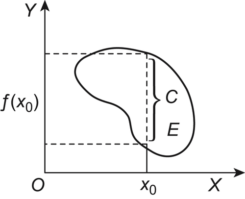
For  , letting
  , we have
  . As shown in Fig. 5.14, via point construct a line perpendicular to X and the intersection of the line and E is set C. Projecting C on Y, we have
  .
.
Obviously,  . When f is single valued, is a graph corresponding to
  and can be regarded as the extension of a general graph.
Characteristic Networks
Definition 5.10
Assume that  is the RMG of A.
  satisfies:
(1)  and its closure
  are arcwise connected sets on D
(2) Let  . Assume that
  has m arcwise connected components on denoted by
  .
.
(3) For  , letting
  , then
  has just m arcwise connected components on denoted by
  and
and  .
.
Then, set is called a homotopically equivalent class of D.
Example 5.4
Solution
Let  and
and  . From the above definition,
  and
and  are homotopically equivalent classes of X, respectively, or and compose a set of homotopically equivalent classes of X.
If  , then D is not a homotopically equivalent class of X. Since
  is simply connected in RMG,
  ,
,  is not connected, i.e., it has two components, D is not a homotopically equivalent class.
If  and
and  , obviously and
  are homotopically equivalent classes of X, respectively.
If  and
and  , then
  and
and  compose a maximal set of homotopically equivalent classes of X. Namely, if E composes a maximal set of homotopically equivalent classes of X, when adding arbitrary element e of X to E and
  , then
  is no longer a set of homotopically equivalent classes of X.
We now construct a characteristic network as follows.
Assume that  and is a graph of f.
(1) R is decomposed into the union of n mutually disjoint regions, and  is a set of homotopically equivalent classes.
(2) Each  has
has  components denoted by
  ,
, 
(3) A set V of nodes composed by  .
.
(4) Nodes  are called neighboring if and only if the components corresponding to
  and
and  have common boundaries on , where
  is the component corresponding to
  .
.
If  then we say that the two components
  and
and  have a common boundary, where
  is the closure of on .
(5) Linking each pair of neighboring nodes of V by an edge, we have a network  . It is called a characteristic network of .
For a state  , x must belong to some component of , i.e., some node v of V. Namely, v is called a node corresponding to the state x. It is denoted by
  . We have the following theorem.
Theorem 5.1
An initial state and a goal state are given. Assume that and correspond to nodes  and
and  , respectively. Then, a rigid body A moves from to without collision if and only if there is a connected path from to on .
Proof
Therefore, we have a finite sequence of points on , namely,
![]() (5.3)
(5.3)
Obviously, both  and
and  belong to
  , and both and
  belong to
  . From the definition of the homotopically equivalent class,
  is arcwise connected. Hence, and belong to the same arcwise connected component. From Proposition 5.4, there exists a collision-free path from to .
To illustrate the construction of the characteristic network, a simple example is given below.
Example 5.5
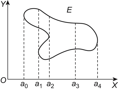
A graph E is shown in Fig. 5.16. We now find its corresponding characteristic network.
Solution
X is divided into the union of three regions and they compose a set of homotopically equivalent classes of X.
![]()
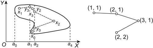
To find the components of each  , we have
Each node corresponding to  is denoted by . Then, we have a network as shown in Fig. 5.16. It is a characteristic network of E.
Given  and
and  , we now find a collision-free path from to . From Fig. 5.16, and belong to nodes
  and
and  respectively. From the characteristic network, we have a connected path:
![]()
From the example, we can see that by the topologic model, the problem of finding a collision-free path in an infinite set is transformed into that of finding a connected path in a finite network so that the computational complexity is reduced.
..................Content has been hidden....................
You can't read the all page of ebook, please click here login for view all page.