7.4. The Expansion of Quotient Space Theory
7.4.1. Introduction
The quotient space theory we have discussed so far is based on the following two main assumptions. (1) The domain structure is limited to topology. (2) The domain granulation is based on equivalence relations, i.e., classification without overlap. Now, we will relax the two restrictions. First, we consider the structures formed by closure operations that are broader than topological ones. Second, domain granulation will be extended from equivalence relations to tolerance relations.
7.4.2. Closure Operation-Based Quotient Space Theory
There is a variety of closure operations, so different structures can be defined by the operations. The domain structures described by closure operations are broader than topological ones generally. For example, the pre-topology defined by closure operations under the Cech’s sense is more universal than well-known topology defined by open sets (Cech, 1966). But the topology defined by Kuratowski closure operation is equivalent to well-known topology.
Now, we introduce some basic concepts about closure space (see Addenda A for more details).
Definition 7.27
Assume that X is a domain. If mapping  :
: satisfies the following axioms, where
  is a power set of X, is called a closure operation on
  , correspondingly
  is called a closure space,
  is a
is a  closure of
  , and for simplicity, is indicated by
  .
.
![]()
![]()
![]()
Proposition 7.6
Assume that is a closure space, then
(1) 
(2)  ,
, , if
, if  , then
(3) For any family  of subsets on ,
  .
.
Definition 7.28
![]()
If  , then
  is called coarser than
  , or is finer than .
Proposition 7.7
Binary relation  is a semi-order relation on
  .
.  has the greatest element
  and the least element
  . For
. For  , if
, if  then
then  , otherwise
  . And for
  ,
,  . Furthermore, any subset
  on and
  ,
,  holds, i.e., is order complete with respect to ‘’.
7.4.2.1. The Construction of Quotient Closure and its Property
![]()
Especially, when is a topological closure operation, the structure decided by  is a corresponding quotient topology on
  .
.
Assume that  and
and  ,
,  is a nature projection, and
  ,
, , is a quotient space having a closure structure, or simply a quotient closure structure. Since ,
  is a nature projection from
  to its quotient set
  .
.  on is a closure operation induced from projection
  with respect to closure operation
  . Thus,
  (Cech, 1966). Generally, the similar result can be obtained for a chain of equivalence relations. Then we have the following proposition.
Proposition 7.8
Assume that  is a chain of equivalence relations on . is a nature projection. ,
  , is a corresponding quotient closure space.
  composes a hierarchical structure, where
  .
.
The similar falsity-preserving principle in closure spaces is the following (Chen, 2005).
Proposition 7.9
If  is a connected subset on , the image
  of under the projection p is a connected subset on
  .
.
Theorem 7.6 (Falsity-Preserving Principle)
From Chapter 1, it’s known that a semi-order relation under the quotient mapping only maintains the reflexivity and transitivity but does not necessarily maintain anti-symmetry generally. For the closure spaces, we will prove that the quasi-semi-order structures are invariant under the quotient mapping (projection), with the help of the continuity of the mapping, but the semi-order structure cannot maintain unchanged under the mapping generally.
Proposition 7.10
Assume that  is a quasi-semi-order space.
  is an equivalence relation on X, and is the corresponding quotient set. Then, there exists a quasi-semi-order
  on such that the nature projection is order-preserving, i.e.,
  , we have
![]()
Proof
Since is a quasi-semi order on X, define an operation induced from as follows
![]()
It’s easy to prove that is a closure operation on X. In fact, is a topologic closure operation with the Alexandroff property. If from closure space define a quasi-semi-order  as
as  , then is the same as . This means that closure operation and quasi-semi order are interdependent.
If  is a quotient closure operation on with respect to , then
  is a topologic closure space. Define a quasi-semi-order
  on as
on as
![]()
Finally, we show that  . In fact, we have
![]()
![]()
![]()
In summary, there exists a quasi-semi-order relation on the quotient structure of a quasi-semi-order space such that the corresponding nature projection is order-preserving.
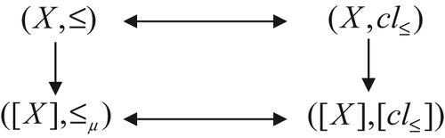
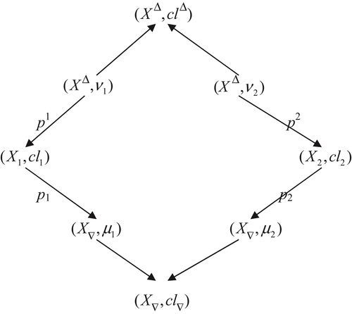
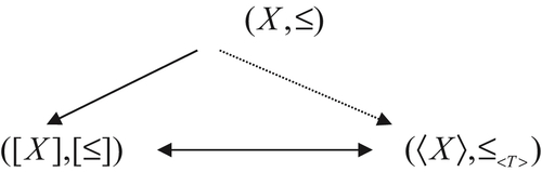
The order-preserving processing processes of quotient closure spaces are shown in Fig. 7.3, where  indicates the closure topology induced from ≤,
  is its corresponding quotient topology, is a quasi-semi-order on [X] induced from ,
  is a quasi-semi-order induced from topology , and [cl] on [X] is a topology induced from cl.
The whole quasi-semi-order relations satisfying reflexivity and transitivity on a domain and the whole Alexandroff topologies on the domain are one–one correspondence. Especially, the whole semi-order relations, i.e., the quasi-semi-order satisfying anti-symmetry as well, and whole Alexandroff topologies satisfying  -separation axiom are one–one correspondence. So the order structure may be regarded as a specific topological structure, and a specific closure structure spontaneously.
Since -separation axiom does not satisfy divisibility, the order relation on quotient space of semi-order space that is constructed by the above method does not have anti-symmetry generally, although its nature projection is an order-preserving mapping. As in Chapter 1, by merging and decomposing, the original equivalence relation R can be changed to R∗ such that corresponding relation satisfies the anti-symmetry in space  .
.
7.4.2.2. The Synthesis of Different Grained Worlds
So far we have shown that a new space can be constructed from given spaces through synthesis methods, when their structure is topologic. We also show that the synthetic space is the least upper bound one, and the projection from the synthetic space on the given spaces plays an important role. In fact, the synthetic principle can be represented as an optimization problem with respect to  , where
  is a projection from the original to quotient spaces,
  and
and  represent the domain, topological structure, or attribute function of the original and quotient spaces, respectively. The synthetic space is either the least upper bound, or the greatest lower bound space among the given spaces. In this section, we will consider the synthetic problem under the closure structures.
Define  .
.  is a quotient set corresponding to
  , and the least upper bound of
  and
and  in partition lattice
  . Both and are quotient sets of .
  are their corresponding projections. It’s easy to show that for each
  , there exists
  such that is projected onto
  by projection
  , and quotient space satisfies the synthetic principle, i.e., is the coarsest partition among all partitions that satisfy . Dually, define
  , where
  denotes the set obtained after implementing transitive operation on elements of X. Quotient space
  corresponding to
  is the greatest lower bound of and in partition lattice . For , is the quotient set of , and its corresponding projection is
  . It’s easy to show that satisfies the synthetic principle, i.e., is the finest partition among all partitions that satisfy
  .
.
According to the synthetic principle,  should be defined as the solution of a set
  ,, of equations. If their solution is not unique, some optimization criteria should be added in order to have an optimal one. Dually,
  should be defined as the solution of a set
  ,, of equations which similar to solving .
A new closure operation can be constructed in the following way, i.e., a new closure operation (or a set of closure operations) can be generated projectively, or inductively by a known mapping (or a set of mappings), respectively. The following proposition shows the relation between the two generation methods.
Proposition 7.11 (Cech, 1966)
First, we consider the construction of closure operation  .
.  is a closure operation on
  that generated projectively by with respect to closure operation
  . Since is a surjection, is generated inductively by with respect to closure operation . Space
  is a quotient closure space of
  with respect to equivalence relation
  . Defining closure operation as
  , then on is the coarsest one among all closure operations that make each
  continuous. Closure space
  is the least upper bound of synthetic spaces
  , but an explicit expression of cannot be obtained generally.
Dually, the construction of closure operation  is as follows.
  is a closure operation on that generated inductively by with respect to closure operation , i.e., is the finest one on among all closure operations that make each
  continuous. Defining closure operation as
  , then is the finest one on among all closure operations that make each continuous. Closure space
  is the greatest lower one of synthetic spaces . The expression of is the following.
The synthetic process of quotient closure spaces can intuitively be shown in Fig. 7.4.
7.4.3. Non-Partition Model-Based Quotient Space Theory
The quotient space theory that we have discussed so far is based on a partition model, i.e., a complete lattice composed by all equivalence relations on a domain, or a partition lattice. The quotient space theory based on the partition model that we called traditional theory is too rigorous. Many real problems do not necessarily meet the requirement, for example, classification with overlap, or with incomplete knowledge, etc. If abandoning the transitivity condition in an equivalence relation, then we have a tolerance relation. Tolerance relation is a broader binary relation than the equivalence one, but still has good attributes. So the tolerance relation-based quotient space theory is a very useful extension of the traditional one.
7.4.3.1. Tolerance Relations
Definition 7.29
Definition 7.30
For  , define
  as a -relevant class of
  , i.e.,
  . The whole is denoted by
  , where
  , for simplicity, and are denoted by
  and
and  respectively, if it does not cause confusion.
Proposition 7.12
If and only if tolerance relation satisfies transitivity, then is a partition of X.
Theorem 7.7
Assume that  is the whole tolerance relations on X, and
  is a set of subscripts.
(1)  and
and  are tolerance relations on X.
(2) Define a binary relation on  as composes a complete lattice with respect to relation , denoted by
  . The intersection operation
  and union operation
  on lattice are defined as follows.
 and
and  are set intersection and union operations, respectively.
![]()
![]()
(3)  ,
,  ,
, 
The proof of the theorem is obvious.
A complete lattice , composed by all tolerance relations on a domain, is similar to a complete lattice  , composed by all equivalence relations on the domain or a partition lattice . Both can be used to describe multi-granular worlds but they are different. In partition, the classes are mutually disjointed. In classification based on tolerance relations the classes do not necessarily mutually disjoint.
7.4.3.2. Tolerance Relation-Based Quotient Space Theory
Definition 7.31
t is a mapping from set to set  . An equivalence relation
  on can be induced from t as follows
![]()
For simplicity, is denoted by  .
.  ,
,  , is an equivalence class with respect to equivalence relation . is the corresponding quotient set, and
  is a nature projection.
Definition 3.30
(1) t is a surjection
(2) for  ,
,  is an open set on
then, Proposition 7.13
t is a quotient mapping from topologic space  to topologic space . is an equivalence relation on induced from t.
  is a quotient topologic space with respect to nature projection . Then, topologic spaces and are homeomorphism, where homeomorphous mapping
  satisfies
  , equivalently,
  .
.
The proposition shows that when  is a quotient mapping, can be regarded as a quotient space of . t is just the corresponding pasting mapping. In fact, quotient spaces and quotient mappings are closely related concepts. The nature projection discussed in Chapter 1 is a specific quotient mapping that satisfies the conditions (1) and (2) in Definition 7.32.
Definition 7.33
t is a surjection from onto . For  , define a topology on as
  . That is,
  is the finest among topologies that make the surjection t from topologic space
  onto
onto  continuous.
Proposition 7.14
t is a quotient mapping from space to . Topologic spaces and  are homeomorphism, where is a pasting space induced from t.
Although is not an equivalence relation, i.e., cannot compose a partition on X, since there is no distinction among homeomorphous spaces in some sense, from Proposition 3.17 it’s shown that the traditional quotient space theory is still available to the tolerance relation. But since the elements on as subsets on X are no longer mutually disjointed, the computational complexity discussed in Chapter 2 will not hold, likely increases.
The construction of quotient attribute  is the same as that of a traditional one. Therefore, if tolerance relation and space
  are given, the quotient space
  can be constructed.
Similar to the traditional theory, we have the following property.
Proposition 7.15
If  is a connected subset on X, then
  is a connected subset on .
Now, we consider the order preserving property. Assume that  on
on  is a quasi-semi-order structure.
  on is an Alexzandroff topology determined by the quasi-semi-order . on is a quotient topology with respect to quotient mapping
  . Define a binary relation
  on as follows
 is an open neighborhood of
  .
.
![]()
Relation is just a specified quasi-semi-order determined by . Since and are homeomorphism, from Proposition 3.13, there exists a quasi-semi-order on such that , if  then
then  . The following proposition shows that quasi-semi-order relation has the order preserving property.
Proposition 7.16
If  and
and  , then
  .
.
Proof
Since and are homeomorphous, the quasi-semi-order on [X] induced from  and the quasi-semi-order on induced from
  are equivalent.
Again from the order preserving of , on has order-preserving as well.
The order-preserving property in tolerance relation-based quotient spaces can be shown in Fig. 7.5 intuitively.
When we discuss the order-preserving property, the homeomorphism of topologic spaces and plays an important role. Similarly, the above homeomorphous relation can still play a significant role in the synthetic problem.
7.4.4. Granular Computing and Quotient Space Theory
Quotient space-based problem-solving theory is a multi-granular computing model under the framework of set theory. We have dealt with the following problems. First, the projection problem is that given a quotient set, to find the representations of attribute and structure on the set, i.e., the descriptions of the coarse-grained world and the relation to the original one. Second, the synthesis problem is that given different views of the world, to find a new understanding of the world based on the known knowledge. Third, the reasoning problem is the reasoning over different grain-size worlds. The final problem is how to choose a proper grain-size world in order to reduce the computational complexity of multi-granular computing.
Now, we discuss granulation and granular computing from the quotient space theory view point.
7.4.4.1. Granule, Granulation and Granular World
In quotient space theory, a ‘granule’ is defined as a subset in a space (domain). In the partition model, the subset is an equivalence class and an element in its quotient space, whose inner structure is determined by the corresponding partition. Each subset can be represented by a complete graph. For example, in a grained level {[1],[4]}={{1,2,3},{4,5}}, element [1] has three components (elements) {1,2,3} and can be represented by a complete graph. Similarly, element [4] has two components {4,5} and can be represented by a complete graph as well. Any two elements are mutually disjointed. In the tolerance relation model, the subset consists of all elements that have tolerance relations. They may have a center that can be represented by a stellate graph. They may have several centers that can also be represented by a stellate graph, when the centers are regarded as a whole. For example, in a grained level {<1>,<2>,<4>,<5>}={{1,2},{1,2,3,4},{2,3,4,5},{3,4,5}}, where ‘bold’ Arabic numerals indicate ‘centers’. Element <1> is a graph with component ‘1’ as a center. Element <4> is a graph with components {3,4} as centers, while components ‘2’ and ‘5’ do not have any connected edge.
In quotient space theory, the granulation criterion is equivalence or tolerance relation. The relation may be induced from attributes, or relevant to them. This is different from the rough set theory. When an equivalence or tolerance relation is given, we have a coarse-grained world. In the world, each element can be regarded as independent; while as subsets in the original domain, they may be mutually disjointed or have an overlapping portion. In addition, a coarse-grained world may have a structure, for example, topologic, closure or order structure. The structure is obtained by a quotient mapping from the original world. The continuity of the quotient mapping plays an important role that we have discussed in previous sections adequately.
7.4.4.2. The Multi-Granular Structure
When a granulation criterion is given, we have a grained world. When several granulation criteria are given, then we have a multi-grained world. What relation exists within the multi-granular world? In other words, what structure the multi-granular world has? In partition model, all equivalence relations compose a complete lattice. Correspondingly, all partitions compose a complete lattice as well. In the tolerance relation model, all tolerance relations compose a complete lattice. Specially, a chain of equivalence relations or tolerance relations is chosen, we have a hierarchical structure. In addition, the existence of complete lattice guarantees the closeness of the newly constructed grained worlds.
7.4.4.3. Granular Computing
In granular computing, the computational and inference object is ‘granules’. Quotient space theory deals with several basic problems of granular computing. For example, considering the computation of quotient attribute functions in a certain grained level, since the arguments of the functions are ‘granules’, their values may adopt the maximum, minimum, or mean of the attribute functions of all elements in the granule. If an algebraic operation is defined on a domain, it’s needed to consider the existence and uniqueness of its quotient operation on a certain grained level. We have discussed this problem in Chapter 4.
The descriptions of a problem in several grain-size worlds are given, how to choose a proper grain-size world to carry out the problem solving? Quotient space theory deals with the problem by information synthesis that mirrors the characteristics of human problem solving, i.e., viewing the same problem from different granularities, translating from one abstraction level to the others freely, and solving the problem at a proper grained level. Information synthesis includes domain, structure and attribute function. Here, the homomorphism principle plays an important role.
Falsity-preserving property is very important in the inference over a multi-granular world. With the help of the continuity of quotient mappings and the connectivity of sets, and considering the structure of domain, the computational complexity can be reduced by multi-granular computing based on quotient space theory.
7.4.5. Protein Structure Prediction – An Application of Tolerance Relations
In the section, we will use the binary relation satisfying anti-reflexivity and symmetry, i.e., equivalent to a tolerance relation, to define the sequence adjacency and topology adjacency in the amino acid sequence folding. Furthermore, we will explain the enhancement method for estimating the lower bound of energy of a protein obtained by the folding of its amino acid sequence, using the concept of tolerance relations.
7.4.5.1. Problem
Protein structure prediction is the prediction of the three-dimensional structure of a protein from its amino acid sequence that is a hot topic in bioinformatics (Martin, 2000). Generally, there are three methods to dealing with the problem, molecular dynamics, protein structure prediction and homology modeling. Different protein models may be established depending on the ways of describing the protein molecular and treating the interaction between amino acid residues and solution. The experimental result for small proteins implies that the primary state of proteins approaches the minimum of free energy. This widely accepted assumption becomes the foundation of protein structure prediction from a given amino acid sequence by means of computation.
Due to the complexity and large scale of protein structure, the simple models are adopted generally. A lattice model is one of the well-known models (Dill et al., 1995). In lattice models, each amino acid residue is represented as an equal size and is confined to regular lattices, the connection between them is assumed to be the same length. For simplicity, 2D rectangle or 3D cuboid lattice point representation of lattice models is adopted. We will only discuss the 2D lattice model below.
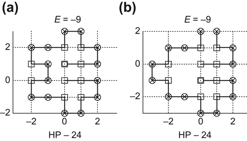
HP lattice model is a representative one (Lau and Dill, 1989, 1990). In the model, amino acids are divided into two categories: hydrophobic (H) and hydrophilic (P). The hydrophilic force is the important driving force behind the folding process. Under the impact of the force, after the folding of the amino acid sequence, the hydrophobic amino acids will concentrate in the center of the protein as far as possible in order for them to keep out of water. In Fig. 7.6(a) the inappropriate folding, (b) the appropriate folding of amino acid sequences are shown.
A sequence  of amino acids is given, where
  ,
,  . After the folding of
  , we have protein
  represented in a 2D-HP model as follows. Amino acids
  and
and  are confined in coordinates
  and
and  , respectively. For
  , the coordinate of
  is represented by the directions of
  relative to
  , i.e., forward, towards the left, and towards the right, respectively. Assume that the interaction of amino acids happens inside a topology adjacent pair, i.e., the amino acids in a pair are adjacent in their lattice but are not adjacent in their sequence. The interaction
  of amino acid pair
  with type
  , or
, or  , is defined as follows respectively.
![]()
The energy of protein obtained by the folding of its amino acid sequence is defined as  , where if and only if
  and
and  are topology adjacent,
  , otherwise
  = 0.
= 0.
An amino acid sequence  with length
  is given. Let
  obtained by the folding of and the hydrophobic amino acids concentrate in the center of }. Under the widely accepted assumption, the protein-folding problem can be represented as follows.
![]()
It has been shown in Nayak et al. (1999) that this is a NP-hard problem. There exists an (or several) optimal solution, or only several sub-optimal solutions.
7.4.5.2. The Estimation of the Lower Bound of Energy
Each anti-reflexive relation corresponds to a reflexive relation uniquely, and vice versa. Correspondingly, each anti-reflexive and symmetric binary relation corresponds to a tolerance relation uniquely. Therefore, in the isomorphism sense, there is no distinction between an anti-reflexive and symmetric binary relation and a tolerance relation.
Assume that  is an amino acid sequence. Protein is obtained from the folding of S, and represented in 2D
  lattice model. For simplicity,
  is indicated by
  .
.
Definition 7.34
Define  as
as  , or
, or  .
.
Definition 7.35
Define  as
as  ,
,  , where
  and
and  represent the horizontal and vertical coordinates of ,
  , in the 2D lattice model, respectively.
Binary relation is an anti-reflexive and symmetric relation on induced from . It indicates the adjacency of two amino acids with respect to sequence, and is called a sequence adjacent relation. In the 2D model, if and only if and satisfy that one of their coordinates is equal and the difference of the other coordinates is 1 unit, then  holds. Obviously,
  satisfies anti-reflexivity and symmetry, and is called a structure adjacent relation.
Now, we define a topology adjacent relation in 2D HP lattice model as follows.
Definition 7.36
Define  as ,
as ,  and
and  .
.
Obviously, the topology adjacent relation is the difference between the structure and sequence adjacent relations, as they can be regarded as a subset on  . In other words,
  , where
  is a complement set of R.
From the widely accepted assumption, the energy of primary state of a protein approaches the minimum. While in the 2D HP lattice model, the hydrophobic amino acids is required to concentrate in its center as far as possible after the folding. Assume that protein P is located in the 2D lattice model with length l and width m, after the folding of an amino acid sequence with length n. In the ideal situation, an amino acid is placed in each lattice point, and the hydrophobic ones are placed in the center lattice points as far as possible. Let  and
and  be the number of elements in set ‘
 ’. Then, satisfies
![]()
While
![]()
![]()
Since
![]()
![]() (7.17)
(7.17)
From and the definition of , if and only if and are topology adjacent, , otherwise =0. Therefore, the Formula (7.17) is the estimation of the lower bound of  , i.e.,
  . The estimation does not eliminate topology adjacent that consists of amino acid pairs with P–P or H–P type. While the interaction among the amino acid pairs either with P–P type or H–P type is zero, and has no effect on the . The lower bound obtained above is not satisfactory. It’s known that only the topology adjacent amino acid pairs with H–H type play a part in . In more ideal cases, the topology adjacent amino acid pairs with H–H type only appear on the rectangle
  that within the rectangle lm. Now, the number of topology adjacent amino acids with H–H type is at most
 .
.
![]()
Let f be the number of amino acid pairs with H–H type in sequence , including the head and the end amino acids of the sequence are H type. We have
![]() (7.18)
(7.18)
This is also a lower bound estimation of .
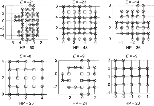
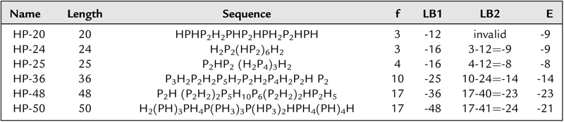
Fig. 7.7 shows the results that are obtained by the folding of HP benchmark sequences in Unger and Moult (1993) via genetic algorithms (GA). The results of the lower bound of energy obtained by genetic algorithms (GA) are shown in Table 7.1.
Table 7.1
The Results of the Lower Bound of Energy via GA
| Name | Length | Sequence | f | LB1 | LB2 | E |
| HP-20 | 20 | HPHP2H2PHP2HPH2P2HPH | 3 | -12 | invalid | -9 |
| HP-24 | 24 | H2P2(HP2)6H2 | 3 | -16 | 3-12=-9 | -9 |
| HP-25 | 25 | P2HP2 (H2P4)3H2 | 4 | -16 | 4-12=-8 | -8 |
| HP-36 | 36 | P3H2P2H2P5H7P2H2P4H2P2H P2 | 10 | -25 | 10-24=-14 | -14 |
| HP-48 | 48 | P2H (P2H2)2P5H10P6(P2H2)2HP2H5 | 17 | -36 | 17-40=-23 | -23 |
| HP-50 | 50 | H2(PH)3PH4P(PH3)3P(HP3)2HPH4(PH)4H | 17 | -48 | 17-41=-24 | -21 |
7.4.6. Conclusions
In the section, we extend the quotient space theory from the aspects of the structure and granulation of a domain. That is, further consider the structure produced by closure operations, and the granulation by tolerance relations. The domain structure plays an important role in quotient space theory, and also is one of the characteristics of the theory. With the help of the continuity of mappings and the connectivity of sets, we have the falsity-preserving property that is very useful in reasoning. The order relation is a specific topological structure. We pay attention to the order-preserving property that is also very useful in reality. Fortunately, these good properties still maintain under the expansion.
..................Content has been hidden....................
You can't read the all page of ebook, please click here login for view all page.