6.3. The Discussion of Statistical Heuristic Search
6.3.1. Statistical Heuristic Search and Quotient Space Theory
The heuristic search generally implements on a tree. A tree is a specific case of a sequence of quotient spaces. If in a sequence of hierarchical quotient spaces, the number of elements in each level is finite, then it’s a tree. Assume that SA implements its search on a uniform m-tree. Let  be the sub-nodes in the first level. From quotient space point of view, it is equivalent to the partition
  of domain
  , where
  is a set of leaf nodes of the subtree rooted at
  . Thus, set
  is a quotient set of the set of the overall leaf nodes. The statistic
  of
of  is extracted from set
  .
.
A heuristic search on a tree or graph can be restated as follows. A statistical heuristic search is sampling on some level (quotient space) of a search space, extracting statistics and making statistical inference on the level. So we can transfer the statistical heuristic search from a tree (graph) to a sequence of quotient spaces.
1. The Quotient Space Model of Heuristic Search
On the other hand, in statistical inference some statistic is used to estimate function  . Thus, the statistical inference method can be used to judging which the solution is.
These mean that we can integrate heuristic search, quotient space method and statistical inference to form a new statistical heuristic search model – a quotient space model of statistical heuristic search.
Assume that  is a set of random variables in a basic probability space
  ,
,  is a sequence of hierarchical quotient spaces of
  , and
, and  are their corresponding equivalence relations, where
  denotes that
  is a quotient space of
  , and
, and  is a finite set.
If  , then
  is partitioned into
  by equivalence relation
  . From
  extracting statistic
  implement statistic inference S based on
  ,…. Where, statistic
  is extracted from a subset of
  , so it represents the global information of the subset.
This is a quotient space model of statistical heuristic search.
6.3.2. Hypothesis I
All conclusions about SA we made are under Hypothesis I. We have a further discussion on the hypothesis.
Hypothesis I
Assume that G is a uniform m-ary tree.  let
let  be a subtree rooted at n. Statistic
  extracted from T(n) (called global statistic) satisfies
(1)  is an i.i.d. random variable having a finite fourth moment,
  is the mean of a(n).
(2)  (L is a solution path),
  ;
;  ,
,  .
.
In essence, this means that the statistics extracted from  should be different from that extracted from
  statistically. In order to apply the statistical inference, in a sense the hypothesis is necessary. But the constraint given in Hypothesis I (2) may be relaxed. Let us examine some relaxed cases.
1. Inconsistent cases
(1) In Hypothesis I, for each  ,
,  and
and  ,
,  , i.e., the above equalities hold consistently. We now may relax the constraints as follows. There exist constants
  and
and  such that for each
  ,
,  ;
;  ,
,  ; and
; and  is finite.
Since  , i.e.,
  is inverse proportion to
  or proportion to
  , where
  ,
,  only depends on the difference between
  and
and  . Therefore, as long as
  , even
  and
and  are changing, the order of the mean complexity of SA does not change any more.
(2) In some cases, although  is less than
  , there does not exist a constant c independent of N such that the former is different from the latter.
We now discuss these kinds of relaxed conditions.
Assume that  and
and  are nodes at the k-th level, where
  . If there exists constant
  such that
  , then for
  subtrees implementing statistical inference S, the order of the complexity is
![]()
Thus, the order of the total complexity of SA is .
.
![]()
The order of mean complexity of SA still remains polynomial. We have the following theorem.
Theorem 6.6
G is a tree.  ,
,  and
and  are nodes at the k-th level, where
  . If there exist constants
  and
and  , such that
  (
( ). Then, the order of total complexity of SA algorithm is
![]()
2. Mixed Cases
‘False Goals': If there are A(N) nodes not belonging to L such that  does not hold, i.e., the global statistics extracted from the subtrees rooted at such nodes do not satisfy
  , then in searching process those nodes statistically are not much different from the nodes belonging to L. There seems to be A(N) 'false goals' in G. The complexity of SA will increase by A(N) times at most. As long as A(N) is a polynomial of N which is the depth the goal is located at, SA can also avoid the exponential explosion.
3.  is not i.i.d
In hypothesis I, it’s assumed that statistic  is i.i.d. and has finite fourth moment. Now, we relax the constraints and only assume that
  is independent and has variance
  , i.e., give up the requirement of the identical distribution
In the proof of the polynomial complexity of SA, we use formulas  and
and  . The above two formulas are based on central limit theorem and Chow-Robbins lemma. However, the precondition of central limit theorem is the i.i.d. assumption of
  . But the i.i.d. assumption is only the sufficient condition but not necessary. In Gnedenko (1956), the central limit theorem is based on the relaxed conditions as shown in Lemma 6.2.
Lemma 6.2
![]() (6.11)
(6.11)
Thus,  , we uniformly have
 (6.12)
The above lemma does not require the identical distribution of  . Then we have the following corollary.
Corollary 6.4
Proof
Since  ,
,  . Let
. Let  . Since
  has finite fourth moment,
  .
.
Substituting the above formula into the left-hand side of Formula (6.11), we have:
![]()
We replace the i.i.d. condition of  by the following conditions, i.e.
  are mutually independent, and have variances
  and finite fourth moments. Similarly, we can revise Chow-Robbins lemma under the same relaxed condition. Since many statistical inference methods are based on the central limit theorem, we have the following theorem.
Theorem 6.7
(1) Random variables  are mutually independent and have variances
  and finite fourth moments.
(2)  and
and  ,
,  , constant
  , where
  and
and  are brother nodes.
Then, the corresponding SA can find the goal with probability one, and the mean complexity  .
.
In the following discussion, when we said that  satisfies Hypothesis I, it always means that
  satisfies the above relaxed conditions.
6.3.3. The Extraction of Global Statistics
When a statistical heuristic search algorithm is used to solve an optimization problem, by means of finding the minimum (or maximum) of its objective function, the ‘mean’ of the statistics is used generally. However, the optimal solution having the minimal (or maximal) objective function does not necessarily fall on the subset with the minimal (or maximal) mean objective function. Therefore, the solution obtained by the method is not necessarily a real optimal solution.
In order to overcome the defect, we will introduce one of the better ways below, the MAX statistic.
1. The Sequential Statistic
We introduce a new sequential statistic and its properties as follows (Kolmogorov, 1950).
Assume that  is a sub-sample with n elements from a population, and their values are
  . Based on ascending order by size, we have
  . If
. If  have values
  then define
  as
as  .
.  is called a set of sequential statistics of
  .
.
Lemma 6.3
Assume that population  has distributed density f(x). If (
  ) is a simple random sample of
  and
and  is its sequential statistic, then its joint distributed density function is
Let X be the maximal statistic of the sub-sample with size n. X has a distributed density function below . From Lemma 6.3, we have
![]()
Definition 6.4
Under the above notions, let:
Lemma 6.4
Assume that  is a simple random sub-sample from a population that has distributed function
  .
.  is its empirically distributed function. Then for a fixed x, ∞<x<∞, we have
![]()
When n→∞, the distributed function  approaches to N(0,1).
2. MAX Statistical Test
Definition 6.5
The MAX1 test with parameter  is defined as follows.
Give  and
and  , X and Y are two random variables. Their observations have upper bounds. Let n be sample size.
  and
and  are their maximal statistics respectively, when using sequential test.
The orders of observations of X and Y are  and
and  , respectively. Assuming that
  , then
  . Let d=k/n.
![]() (6.13)
(6.13)
If  , stop and the algorithm fails.
Otherwise,
![]() (6.14)
(6.14)
If n<N′, the observation continues.
Definition 6.6
The MAX2 test with parameter  is defined as follows.
In the definition of MAX1 test, the statement ‘If  , stop and the algorithm fails’ is replaced by ‘If
  , when
  we may conclude that the maximum of X(Y) is greater than the maximum of Y(X)’, then we have MAX2 test.
Definition 6.7
If in the i-level search of SA, the MAX1 (or MAX2) with parameter  is used as statistical inference method, then the corresponding SA search is called SA(MAX1) (or SA(MAX2)) search with significant level
  (
( ) and precision
  .
.
3. The Precision and Complexity of MAX Algorithms
Lemma 6.5 (Kolmogorov Theorem)
Lemma 6.6
Assume that  is the empirically distributed function of
  and
and  is continuous. Given
  , then when
  , we have
![]()
Proof
When  , we have
  , i.e.
  .
.
Proposition 6.1
X and Y are two bounded random variables and their continuously distributed functions are  and
and  , respectively. Their maximums are
  and
and  respectively, where
  . Let
. Let  . Assume that
  . Given
  , let
, let
Thus, if  and
and  , then we can judge that the maximum of X(Y) is greater than the maximum of Y(X) with probability
  .
.
Proof
Since  is continuous and
  . Assume that the corresponding orders of observations of X and Y are
  and
and  , where
  , then we have
  . Let
. Let  and
and  .
.
When  , we have
![]() (6.15)
(6.15)
Thus, when  from Formulas (6.16) and (6.17), the correct rate of the judgment is
  , and the computational complexity is
  .
.
In fact, the value of  is not known in advance, so in MAX1 test we replace
  by
by  . This will produce some error. In order to guarantee
  , we may replace
  in Formula (6.13) by the following value
![]() (6.18)
(6.18)
Corollary 6.5
Under the assumption of Proposition 6.1, the correct rate of judgment by MAX1 test is  , and its complexity is
  .
.
4. The Applications of SA(MAX) Algorithms
The SA search based on statistical inference method MAX is called SA(MAX) algorithm. In the section, we will use SA(MAX) to find the maximum of a function.
Assume that  is a measurable function, where D is a measurable set in an n-dimensional space. The measure of D is
  , a finite number. Assume that
  .
.
Regarding  as a measure space, define a random variable
  from
from  as follows.
![]()
When using SA(MAX) algorithm to find the maximum of functions, the given requirement is the following.
(1)  , where c is a given positive number.
(2) When D is finite,  , generally let c=1.
Now, we consider the precision and complexity of SA(MAX) algorithm in the finding of the maximum of functions.
Theorem 6.8
Proof
If the algorithm succeeds, i.e. the judgment of MAX1 succeeds at every time, then the correct probability of judgment at every time is greater than  . The total correct probability is greater than
  .
.
The algorithm is performed through L levels. The total complexity of SA(MAX) is  .
.
Theorem 6.9
Under the same condition as Theorem 6.8, given  and
and  , SA(MAX2) algorithm with parameter
  at each level is used to find the maximum of function f. When algorithm terminates, we have the maximum
  ; the probability of
  , or
, or  , is greater than
  , and the order of complexity is
  .
.
Proof
Similar to Theorem 6.8, we only need to prove the  case. Assume that when the search reaches the i-th level
  , and we find the maximum
  . From Proposition 6.1, we have that the probability of
  is greater than
  . On the other hand,
  is a monotonically increasing function with respect to
  . Let
. Let  . We further have that the probability of
  is greater than
  .
.
Since the complexity at each level is  . The complexity for L levels search is
  at most.
From Theorem 6.9, it’s known that different from SA(MAX1) algorithm SA(MAX2) never fails, but the conclusion made by SA(MAX2) is weaker than SA(MAX1). Secondly, since constants  and
and  can be arbitrarily small, the maximum can be found by SA(MAX2) with arbitrarily credibility and precision.
5. Examples
For comparison, SA(MAX) and GA (Genetic Algorithm) algorithms are used to solve the same problem (Zhang and Zhang, 1997a, 1997b).
Example 6.1
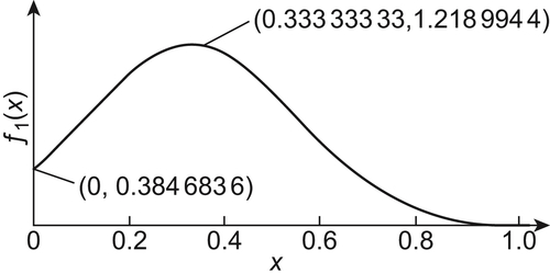
The goal is to find the maximum of function  (Fig. 6.2).
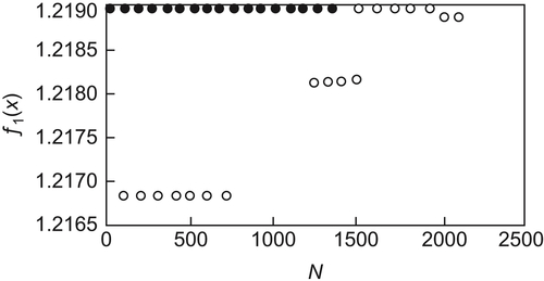
The relation between the results obtained by the two algorithms and N is shown in Fig. 6.3, where N is the total times of calculating function  . The ‘black dots’ show the results obtained by SA(MAX) algorithm when N=64, 128,…. We can see that the maximum of
  obtained by the algorithm in each case is the real maximal value. The ‘white dots’ show the results obtained by GA algorithm when N=100, 200,…. We can see that the best result obtained by the algorithm is the value of
  at x=0.3333216.
Example 6.2
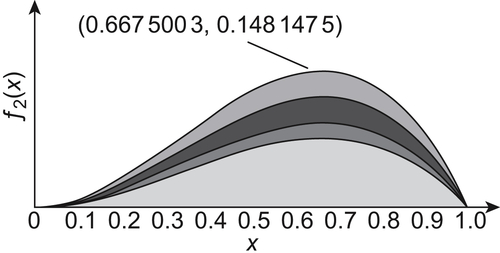
The goal is to find the maximum of function  (Fig. 6.4).
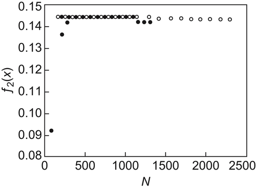
The ‘black dots’ and ‘white dots’ in Fig. 6.5 show the results obtained by SA(MAX) and GA algorithms, respectively. The maximum obtained by SA(MAX) is 0.1481475 (x=0.6675003). In GA, the iteration is implemented for 20 generations and each generation has 100 individuals. The maximum obtained is 0.1479531 (x=0.6624222).
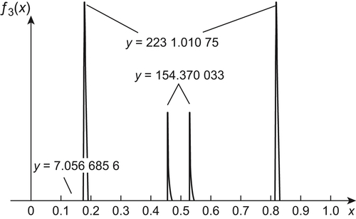
Example 6.3
The goal is to find the maximum of  (Fig. 6.6).
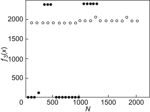
The results are shown in Fig. 6.7. We can see that SA(MAX) finds two maximums of  , i.e., 2231.01075, x=0.1749125 and 2231.01075, x=0.8250875, but GA finds only one maximum of
  , i.e., 2052.376 , x=0.8246953.
From the above results, it’s known that the performances of SA(MAX) are better than that of GA.
6.3.4. SA Algorithms
In statistical heuristic search, the statistic inference method is introduced to heuristic search as a global judgment for subsets so that the search efficiency is improved. Under a given significant level, if a search direction is accepted by SA, the probability for finding the goal can be ensured. When a wrong direction is chosen, SA will terminate with the polynomial mean complexity at most. By using successively SA search the goal can be found with probability one and with polynomial complexity. In fact, in the new round search, a new significant level or a new statistic inference method may be used, based on the results obtained in the previous round. So a variety of SA algorithms can be constructed.
Now, we summarize the SA procedure as follows.
If a statistic inference method S and a heuristic search algorithm A are given then we have a SA algorithm.
(1) Set up a list OPEN of nodes. Expand root node  , we have m sub-nodes, i.e., m
  -subtrees or m equivalence classes in some quotient space. Put them into m sub-lists of OPEN, each corresponds to one
  -subtree. Set up closed list CLOSED and waiting list WAIT. Initially, they are empty. Set up a depth index i and initially i=1.
(2) LOOP. If OPEN is empty, go to (11).
(3) From each sub-list of OPEN choose a node and remove it from OPEN to CLOSED. And call it node n.
(4) If n is a goal, success.
(5) Expand node n, we have m sub-nodes and put them into OPEN. Establish a pointer from each sub-node to node n. Reorder nodes in sub-lists by the values of their statistics. Perform statistical inference S on each sub-list, i.e. sub-tree.
(6) If some  -subtree T is accepted. Remove the rest of
  -subtrees accept T from OPEN to WAIT, go to (10) .
(7) If no  -subtree is rejected, go to LOOP.
(8) Remove the rejected  -subtrees from OPEN to WAIT.
(9) If there is more than one  -subtree in OPEN, go to LOOP.
(10) Index i is increased by 1  . Repartition
  -subtree on OPEN into its sub-subtrees and reorder the sub-aubtrees based on their statistics. Go to LOOP.
(11) If WAIT is empty, fail.
(12) Remove all nodes in WAIT to OPEN, let  and go to (10)
..................Content has been hidden....................
You can't read the all page of ebook, please click here login for view all page.