Chapter 6
Statistical Heuristic Search
Abstract
Heuristic search is a graph search procedure which uses heuristic information from sources outside the graph. But for many known algorithms, the computational complexity depends on the precision of the heuristic estimates, and for lack of global view in the search process the exponential explosion will be encountered when the node evaluation function estimated is not very precise. Based on the similarity between the statistical inference and heuristic search, we consider a heuristic search as a random sampling process, and treat evaluation functions as random variables. Once a searching direction is chosen, it's regarded as if making a statistical inference. By transferring the statistical inference techniques to the heuristic search, a new search method called statistical heuristic search algorithm, SA for short, is obtained. The procedure of SA is divided into two steps hierarchically. First it identifies quickly the most promising subpart (sub-tree) of a search graph by using some statistical inference method. The sub-trees which contain the goal with lower probability are rejected (pruned). The most promising one is selected. Second, it expands nodes within the selected sub-tree using some common heuristic search algorithm. These two steps are used alternately. The statistical heuristic search can be regarded as one of the applications of multi-granular computing.
Due to the combination of different statistical inference and heuristic search methods, different kinds of statistical heuristic search algorithms can be obtained. The SPA algorithms, the combination of the Wald sequential probability ratio test method and best first search algorithm, the SAA algorithms, the combination of asymptotically efficient sequential fixed-width confidence estimation of the mean and best first search, etc. are presented.
Their computational complexity, the comparison to other search methods and weighted techniques are discussed. The extension to AND/OR graph search is also discussed.
Keywords
computational complexity; graph search; heuristic search; statistical heuristic search; statistical inferenceChapter Outline
6.1 Statistical Heuristic Search
6.1.1 Heuristic Search Methods
6.1.3 Statistical Heuristic Search
6.2 The Computational Complexity
6.2.4 The Successive Algorithms
6.3 The Discussion of Statistical Heuristic Search
6.3.1 Statistical Heuristic Search and Quotient Space Theory
6.3.3 The Extraction of Global Statistics
6.4 The Comparison between Statistical Heuristic Search and Algorithm
6.4.2 Comparison to Other Weighted Techniques
In computer problem solving, we know that many types of real problems are conveniently described as a task of finding some properties of graphs. Recall that a graph consists of a set of nodes, which represent encodings of sub-problems. Every graph has a unique node s called the root node, representing the initial problem in hand. Certain pairs of nodes are connected by directed arcs, which represent operators available to the problem solver. If an arc is directed from node n to node p, node p is said to be a successor of n and node n is said to be a father of p. The number of successors emanating from a given node is called the branching factor (or branching degree) of that node, and is denoted by m. A sequence  of nodes, where each
  is a successor of
  , is called a path from node
  to node
  with length k. The cost of a path is normally understood to be the sum of the costs of all the arcs along the path.
A tree is a graph in which each node (except one root node) has only one father. A uniform m-ary tree is a tree in which every node has the same branching factor m.
Now, we consider a problem in hand that is incomplete knowledge or highly uncertain. In order to solve the problem, the search means is generally adopted, i.e., to search the solution in a problem solving space or a search graph. Thus, search is one of the main fields in artificial intelligence. If the size of the space is small, the exhaustive and blind search strategy can be adopted. But if the space becomes larger some sort of heuristic information should be used in order to enhance the search efficiency.
Heuristic search is a graph search procedure which uses heuristic information from sources outside the graph. Some heuristic search algorithms, for example  , have been investigated for the past thirty years. In those algorithms, taking BF (Best-First) for example, the promise of a node in a search graph is estimated numerically by a heuristic node evaluation function
  , which depends on the knowledge about the problem domain. The node selected for expansion is the one that has the lowest (best)
  among all open nodes.
But for many known algorithms, the computational complexity depends on the precision of the heuristic estimates, and for lack of global view in the search process the exponential explosion will be encountered when the node evaluation function estimated is not very precise. For example, Pearl (1984a, 1984b) made a thorough study about the relations between the precision of the heuristic estimates and the average complexity of  , and it is confirmed that a necessary and sufficient condition for maintaining a polynomial search complexity is that
  be guided by heuristics with logarithmic precision. In reality, such heuristics are difficult to obtain.
Based on the similarity between the statistical inference and heuristic search, we consider a heuristic search as a random sampling process, and treat evaluation functions as random variables. Once a searching direction is chosen, it's regarded as if making a statistical inference. By transferring the statistical inference techniques to the heuristic search, a new search method called statistical heuristic search algorithm, SA for short, is obtained. Some recent results of SA search are presented in this chapter (Zhang and Zhang, 1984, 1985, 1987, 1989a, 1989b).
In Section 6.1, the principle of SA is discussed. The procedure of SA is divided into two steps hierarchically. First it identifies quickly the most promising subpart (sub-tree) of a search graph by using some statistical inference method. The sub-trees which contain the goal with lower probability are rejected (pruned). The most promising one is selected. Second, it expands nodes within the selected sub-tree using some common heuristic search algorithm. These two steps are used alternately.
In Section 6.2 the computational complexity of SA is discussed. Since a global judgment is added in the search, and the judgment is just based on the difference rather than the precision of the statistics extracted from different parts of a search graph, the exponential explosion encountered in some known search algorithms can be avoided in SA. It's shown that under Hypothesis I, SA may maintain a polynomial mean complexity.
In Section 6.3, in order to implement a global judgment on sub-trees, the subparts of a search graph, information which represents their global property should be extracted from the sub-trees. The extraction of global information is discussed. Moreover, both global information extraction and statistic heuristic search process will be explained by the quotient space theory.
In Section 6.4, Hypothesis I is compared with the conditions which induce a polynomial mean complexity of A∗. It indicates that, in general, Hypothesis I which yields a polynomial mean complexity of SA is weaker than the latter.
In Section 6.5, from the hierarchical problem solving viewpoint, the statistical heuristic search strategy is shown to be an instantiation of the multi-granular computing strategy.
6.1. Statistical Heuristic Search
6.1.1. Heuristic Search Methods
1. BF Algorithm
Assume that G is a finite graph,  is a node and
  is a goal node in G. Our aim is to find a path in G from
  to
to  . We regarded the distance between two nodes as available information and define its distance function
  as
as is the shortest path from
  to n
to n
![]()
Define  as
as is the shortest path from n to
![]()
Let  .
.  is the evaluation function of
  , denoted by
  , where
  and
and  are evaluation functions of
  and
and  , respectively.
Property 6.1
If there exists a path from  to
to  and algorithm
  can find the shortest path from
  to
to  , then
  is called admissible.
If  has the following constraint, i.e.,
  ,
,  , where
  is the path from
  to
to  ,
,  is called monotonic.
Property 6.2
If  is monotonic, when
  expands any node n, we always have
  .
.
Property 6.3
If  is monotonic then the values of
  corresponding to the sequence of nodes that expanded by
  are non-decreasing.
Obviously, if the values of  are strictly increasing, then the nodes expanded by
  are mutually non-repeated.
2. The Probabilistic Model of Heuristic Search
Nilsson (1980) presented  algorithm and discussed its properties. Pearl (1984a, 1984b) from probabilistic viewpoint, analyzed the relation between the precision of the heuristic estimates and the average complexity of
  comprehensively.
Pearl assumes that a uniform  ary tree G has a unique goal node
  at depth N at an unknown location.
  algorithm searches the goal using evaluation function
  ,
,  , where
  is the depth of node n,
  is the estimation of
  , and
, and  is the distance from n to
  . Assume that
  is a random variable ranging over
  and its distribution function is
 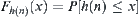 .
.  is the average number of nodes that expanded by
  , until the goal
  is found, and is called the average complexity of
  .
.
One of his results is the following.
Property 6.4
If  has a typical error of order
  and
and  , then the mean complexity of the corresponding
  search is
  , where c is a positive constant.
From Property 6.4, it’s known that if  is estimation with a typical error of order
  , then the mean complexity of
  is greater than
  , where k is a given positive integer. This means that the mean complexity of
  is not polynomial.
Corollary 6.1
If  is an estimation function with a typical error of order
  , then the necessary and sufficient condition that
  has a polynomial mean complexity is that
  is a function with logarithmic order.
A specific case: if there exist  and
and  such that
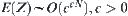
![]() (6.3)
(6.3)
Formula (6.3) shows that so long as the probability that the relative error of  is greater than any positive number is greater than
  , the complexity of
  is exponential. So the exponential explosion of
  search cannot be avoided generally, since it is already difficult to make the function estimation less than very small positive number moreover less than any small positive number.
It is difficult to avoid the exponential explosion for  search. The reason is that the global information is not to be fully used in the search. The complexity of
  search depends on the accuracy of the evaluation function estimation; the accuracy requirement is too harsh. Actually, the information needed in search is only the distinction of evaluation functions between two types of paths containing and not containing goal node, while not necessarily needing the precise values. So the ‘distinction’ is much more important than the ‘precision’ of evaluation function estimation. We will show next how the statistical inference methods are used to judging the ‘distinction’ among search paths effectively, i.e., to decide which path is promising than the others based on the global information.
6.1.2. Statistical Inference
Statistical inference is an inference technique for testing some statistical hypothesis - an assertion about distribution of one or more random variables based on their observed samples. It is one major area in mathematical statistics (Zacks, 1971; Hogg et al., 1977).
1. SPRT Method
The Wald Sequential Probability Ratio Test or SPRT method is follows.
Assume that  is a sequence of identically independent distribution (i.i.d.) random variables.
  is its distributed density function. There are two simple hypotheses
  and
and 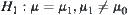 . Given n observed values, we have a sum:
![]()
According to the stopping rule, when  the sampling continues, if
  , hypothesis
  is accepted and the sampling stop at the R-th observation; if
  , hypothesis
  is accepted, where a and b are two given constants and
  .
.
The SPRT has the following properties.
Property 6.5
If hypotheses  and
and  are true, then the probability that the stopping variable R is a finite number is one.
Property 6.6
If 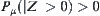 , then
 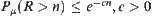 , where R is a stopping random variable of the SPRT, where
  .
.
Property 6.7
Given a significance level , letting
  ,
,  ,
,  and
and  . If
. If  , then the mean of stopping variable, the average sample size, of SPRT is
![]() (6.4)
(6.4)
![]()
![]()
![]()
If the distribution of the random variable is normal, then the stopping rule of SPRT is as follows. and
and  . The Type I error is
  . The Type II error is
  . Type I error means rejecting
  when it is true. Type II error means that when
  is true but we fail to reject
  .
.
 (6.5)
(6.5)
2. ASM Method
Asymptotically Efficient Sequential Fixed-width Confidence Estimation of the Mean, or ASM, is the following.
Assume that  is a sequence of identically independent distribution (i.i.d.) random variables and its joint distributed density function is F,
  , where
  is a set of distribution functions with finite fourth moments. Given
  and
and  , we use the following formula to define stopping variable
  , i.e.,
  is the minimal integer that satisfies the following formula
 and
and 
![]() (6.6)
(6.6)
Let  be the mean of
  . The following theorem holds.
Property 6.8
Property 6.9
If  , then we have
  and
and 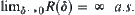 , where
  indicates almost surely, or almost everywhere.
Property 6.10
![]() (6.7)
(6.7)
Property 6.11
![]() (6.8)
(6.8)
Both Formulas (6.4) and (6.8) provide the order of the mean of stopping variable, i.e., the order of the average sample size. In Pearl’s probabilistic model, the average complexity of a search algorithm is the average number of nodes expanded by the algorithm. If we regard a heuristic search as a random sampling process, the average number of expanded nodes is just the average sample size. Therefore, Formulas (6.4) and (6.8) provide useful expressions for estimating the mean computational complexity of search algorithms.
6.1.3. Statistical Heuristic Search
1. The Model of Search Tree
Search tree G is a uniform  ary tree. There are root node
  and unique goal node
  at depth N. For each node p at depth N, define a value
  such that
 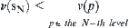 , where
  are goal nodes. Obviously, if
 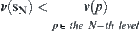 , then
  is a unique goal node.
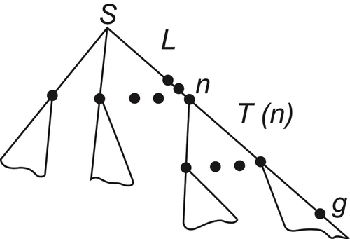
For any node n in G,  represents a sub-tree of G rooted at node n. If n locates at the i-th level,
  is called the
  subtree (Fig. 6.1).
When search proceeds to a certain stage, the subtree  composed by all expanded nodes is called expanded tree.
  is the expanded subtree in
  .
.
Heuristic information: For  ,
,  is a given function value. Assume that
  is the estimation of
 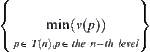 . Therefore, the procedure of
  (or BF) algorithm is to expand the nodes that have the minimal value of
  among all open nodes first.
. Therefore, the procedure of 2. Statistic(an)
In order to apply the statistical inference methods, the key is to extract a proper statistic from  . There are several approaches to deal with the problem. We introduce one feasible method as follows.
Fixed  , let
, let  be an expanded tree of
  and k is the number of nodes in
  . Let
. Let .
.
![]() (6.9)
(6.9)
When a node of  is expanded, we have a statistic
  . When we said that the observation of a subtree in
  is continued, it means that the expansion of nodes in
  is continued, and a new statistic
  is calculated based on Formula (6.9).
  is called a new observed value.
Assumption I
For any  ,
,  is assumed to be a set of identically independent random variables. Let L be a shortest path from
  . If
. If  , then
  ; while
  , then
  , where
  is the mean of
  .
.
In the following discussion, if we say ‘to implement a statistical inference on subtree T’, it means ‘to implement a statistical inference on statistic  corresponding to T’.
  is called a statistic of a subtree, or a global statistic.
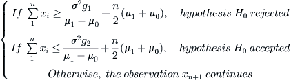
3. SA Algorithm Routine
Given a hypothesis testing method S, introducing the method to a heuristic search algorithm A, then we have a statistical heuristic search algorithm SA. Its routine is the following.
Step 1: expand the root node  , we have m successors, i.e., 0-subtrees. The subtrees obtained compose a set U.
Step 2: Implement statistical inference S on U.
(1) If U is empty, algorithm SA fails. It means that the solution path is deleted mistakenly.
(2) For each  subtree in U, expand node n that has the minimal value of
  among all expanded nodes. If there are several such nodes, then choose one that has the maximal depth. If there are still several nodes at the maximal depth, then choose any one of them. The newly expanded nodes are put into U as the successors of each subtree. Then implement a statistical inference on each subtree in U.
(a) When a node at depth N is encountered, if it’s a goal node then succeed; otherwise fail.
(b) If the hypothesis is accepted in some i-subtree T, then all nodes of subtrees are removed from U except T. the subtree index  and go to Step 2.
(c) If the hypothesis is rejected in some i-subtree T, then all nodes in T are removed from U and go to Step 2.
(d) Otherwise, go to Step 2.
In fact, the SA algorithm is the combination of statistical inference method S and heuristic search BF. Assume that a node is expanded into m sub-nodes  . A subtree rooted at
  in the i-th level is denoted by i-
 , i.e., i-subtree. Implementing the statistical inference S over i-subtrees
  , prune away the i-subtrees with low probability that containing goal g and retain the i-subtrees with high probability, i.e., their probability is greater than a given positive number. The BF search continues on the nodes of the reserved sub-tree, e.g., i-
 . That is, the search continues on the (i+1)-subtrees under i-
 . The process goes on hierarchically until goal g is found.
Obviously, as long as the statistical decision in each level can be made in a polynomial time, through N levels (N is the depth at which the goal is located), the goal can be found in a polynomial time. Fortunately, under certain conditions SPRT and many other statistical inference methods can satisfy such a requirement. This is just the benefit which SA search gets from statistical inference.
..................Content has been hidden....................
You can't read the all page of ebook, please click here login for view all page.