1.5. Property-Preserving Ability
1.5.1. Falsity-Preserving Principle
We have discussed the relation between the domains [X] and X. For a problem space (X, f, T,), structure T is very important. When a domain X is decomposed, its structure will change as well. Generally, it is simplified. The main point is whether some properties (or attributes) in X that we are interested in are still preserved after the simplification.
Generally speaking, there is a wide variety of structures. It is difficult to make a general discussion. We'll focus our attention on two common cases, i.e., topologic structure and semi-order structure. Although semi-order is one of topologic structures, due to its particularity we still discuss them separately.
1.5.1.1. Structure and Quotient Structure Analysis
(1). Topologic Space (X, f, T)
We first introduce some basic concepts of topology below. Readers who are not familiar with them are referred to (Eisenberg, 1974; Sims, 1976).
Definition 1.17
Assume that X is a set. T is a family of subsets on X. If T satisfies
(1) 
(2) If  , then
(3) If  , then
  , where I is an index set, the potential of I is arbitrary.
T is a topology on X. (X, f, T) is a topologic space. For  , if
, if  , then u is said to be an open set.
Example 1.9
Let X={a,b,c,d} and  . T is a topology on X.
If a topology is given on X, then the inner-relational structure T among the elements of X will be defined. Since the relationship among the elements in many domains can be described by topologic structure, topology is a useful tool in problem solving and granular computing. In fact, different topologies can be defined on the same domain X, i.e., the topology of X is not unique.
Definition 1.18
Assume that (X, f, T) is a topologic space. B is a family of sets on X and satisfies
(1) 
(2)  , there exists a subset
  of B such that
B is called a base of (X, f, T).
In Definition 1.18, the condition (1) shows that B is composed by open sets and (2) shows that any open set on X can be represented by the union of some sets of B.
Example 1.10
Assume that X is a one-dimensional Euclidean space. Letting  , then B is a base of X, where
  denotes an open interval.
For a domain X, when its base is confirmed, its corresponding topology is uniquely decided. Contrary, although topology T is decided on X, it can have different bases.
Assume that R is an equivalence relation on X. From R, we have a quotient set [X]. A topology [T] on [X] induced from T is defined as follows.
![]()
[T] is said to be a quotient topology. ([X], [T]) is a quotient topologic space. In addition, p: X → [X] is a natural projection that is defined as follows:
![]()
Quotient structures have a clear geometric interpretation. If an element of [X] is regarded as a subset of X, then a subset of [X] is a set of X. When a subset of [X] is an open set of X, then the subset is defined as an open set on [X], and vice versa. In other words, an open set of [X] is merged by elements of [X] and is also an open set of X.
Example 1.11
Let X={1,2,3,4,5},  . T is a topology on X.
Assuming  , we have
 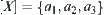 .
.
From the above definition, we obtain
Thus, 
Example 1.12
(X,T) is a two-dimensional Euclidean plane  . Topology T is defined by Euclidean distance.
If choosing equivalence relation R as follows:  ,
, , then we have a corresponding quotient space ([X],[T]) that is homeomorphous to
  .
.
The geometric intuition of the above equivalence transformation is the following. If all points of the line that are perpendicular to x axis at point  are regarded as an equivalence class, then we have a quotient space ([X],[T]), where each element of [X] corresponds to a point of x axis, and quotient topology [T] corresponds to Euclidean distance on x axis.
Example 1.13
In an electronic instrument, if its elements such as resistors, capacitors and integrated circuits, etc., compose a domain X, then the circuit consisting of these elements is a structure T of X. If some elements of X with similar function are classified and designated as components, for example, power supply, amplifier, etc., and the components are regarded as new elements, we then have a new domain [X]. The block diagram consisting of these components is a structure [T] of [X]. It turns out a simplified ‘circuit’ of the original one.
From topology (Eisenberg, 1974), it's known that some properties of the original topologic space (X, T) can still be preserved in its quotient space ([X],[F]). We have:
Proposition 1.3
Natural projection p from (X, T) to ([X], [T]) is a continuous mapping. If  is a connected set on X, then p(A) is a connected set on [X].
This means that in some cases the connectivity is invariant under the grain-size change.
In reality, the solution to some problems can be found by considering the connectivity of a set. From Proposition 1.3, it shows that if there is a solution path (connected) in the original domain X, then there exists a solution path in its properly coarse-grained domain [X]. Conversely, in a coarse-grained domain, if a solution path does not exist, there is no solution path in its original domain. These properties are very useful in practice.
Taking motion planning of a robotic arm as an example, when its environment is rather complicated, the complexity would result in it being computationally intractable if one tries to find a collision-free path for the arm with the geometric details of the environment all at once. Based on topological approaches, the geometric space can be divided into several homotopically equivalent regions. That is, each region has the same topologic structure. We view each as an equivalence class, ignoring all the geometric details within the regions. Then, the original geometric space will be transformed to a network with a finite number of nodes which consist of these regions. From topology, it's known that the connectivity of the network is the same as that of the original space, although the original space has been greatly simplified. In other words, the network, called characteristic net, is a quotient space of the original space, which preserves the connectivity as the original one.
Instead of one step planning, the motion planning may be hierarchically decomposed into two steps. First, it identifies quickly the possible collision-free paths on the characteristic network. Then, it refines the path within the original space based on some given requirements. From Proposition 1.3, it's known that since the regions which have no collision-free paths have been pruned off in the first step, the complexity of the motion planning in the second step is greatly reduced. So, the total complexity of motion planning is improved. A more detailed discussion of the approach will be presented in Chapter 5.
(2). Semi-Order Space (X, T)
(X, T) is a semi-order space, if there exists a relation < among a part of elements on X such that
![]()
If only condition (2) holds, (X, T) is called a pseudo semi-order space.
In order to establish some relations between semi-order spaces at different grain sizes, we expect to induce a structure [T] of [X] from T of X such that ([X], [T]) is also a semi-order space and for all  , if x < y then [x] < [y]. Namely, it is desired that the order relation is preserved invariant under the grain-size change, or order-preserving for short.
It needs several steps to reach the goal.
(1) Transform (X, T) into some sort of topologic space,
(2) Construct a quotient topologic space ([X], [T]) from (X, T), and
(3) Induce a semi-order from ([X], [T]) such that the original order relations are preserved in the quotient space.
Definition 1.19
Assume (X, T) is a semi-order space, for , we define a set 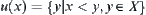 .
.
Let 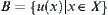 . The topology Tr with B as its base is said to be a right-order topology of X. Hence, a semi-order space is transformed to a topologic space (X,Tr).
Assume that [X] is a quotient set of X. ([X], [Tr]) is a quotient space with respect to (X,Tr).
One of the main properties of the right-order topology is stated as follows.
Property 1.1
(X,T) is a semi-order space. Tr is a right-order topology induced from T. Then,  , there exists a minimal open set u (x) containing x, where
  .
.
Conversely, if there is a topology T satisfying T0-separation axiom such that for all there exists a minimal open set  , then a semi-order Ts on X can be induced from T by the following approach. And T is just the right-order topology of Ts, i.e.,
  , where u(x) is a minimal open set containing x.
Note that a topologic space (X,T) is said to be T0-separation, if for all  , either there exists a neighborhood u(x) of x such that
  or there exists a neighborhood u(y) of y such that
  .
.
Definition 1.20
Assume (X, T) is a topologic space, we define a relation < by T as follows. For  , where u(x) is an open neighborhood of x. The topology Ts corresponding to relation ‘<’ obtained above is called the induced (pseudo) semi-order from T.
The relation ‘<’ defined by Definition 1.20 always satisfies the transitivity but generally does not satisfy the condition:  .
.
Definition 1.21
(X,T) is a topologic space. If the relation ‘<’ defined by Definition 1.18 satisfies the condition: , topology T is said to be compatible with relation ‘<’.
If a relation ‘<’ is compatible with T of (X,T), then relation ‘<’ is a semi-order and X is a semi-order set under relation ‘<’. (X,Ts) is a semi-order space corresponding to (X,T). Sometimes, it is also denoted by (X,T) for short.
Suppose that (X,T) is a semi-order space. [X] is a quotient set of X with respect to R. Tr is a right-order topology induced from T. If topology [Tr] of quotient topologic space ([X],[Tr]) is compatible with the relation ‘<’ defined by Definition 1.20, R is said to be compatible with T, or simply, R is compatible, ([X],[Tr]s) ( or ([X],[Tr])s) is a semi-order space under relation ‘<’ and is denoted by ([X],[T]) for short. It is a quotient structure induced from the semi-order space (X,T) and has the order-preserving ability. If R is not compatible with relation ‘<’, ([X],[Tr]s) is a pseudo semi-order space.
Example 1.14
Whether there exists a quotient semi-order in  ; the answer is the following.
(1) right-order topology Tr induced from T
(2) quotient topology [Tr] on induced from Tr
Thus 
(3) semi-order [T]s induced from [Tr]
From Definition 1.19, we obtain
![]()
Obviously, R is compatible with T. [T]s is a semi-order on and
If  and
and  , then
![]()
Hence, [F]s is not a semi-order on  . R2 is not compatible with T.
Now, we consider some useful properties of ([X],[T]) and (X,T) below.
Proposition 1.4
Suppose that R is compatible with T. If  and x < y, then [x]<[y], where
  .
.
Proof:
Assume x<y. Let a=[x]. u(a) is whichever open neighborhood of a on [X]. Since  is continuous,
  is an open set on X, i.e., a neighborhood of x.
And  , we have
  .
.
Proposition 1.4 indicates that the quotient (pseudo) semi-order space constructed by the preceding approach has the order-preserving ability.
Proposition 1.5
Assume that R is compatible. If  and x<y, then interval
  .
.
Proof:
From  and Proposition 1.4, we have
  . Since
  , from the compatibility of R, we have
  .
.
Definition 1.22
(X,T) is a semi-order set. A 
 is connected

 ,
, 
 A,
A,  =
=  ,
,  ,…,
,…,  =, such that
  and
and  , i = 1,2,…, n-1, are compatible.
Definition 1.23
(X,T) is a semi-order set. A is a semi-order closure if  , and
, and  , then interval
  .
.
Corollary 1.1
In assuming that R is compatible, each component of [X] must consist of several semi-order closed, mutually incomparable, and connected sets.
Note that sets A and B are mutually incomparable, if for  , x and y are incomparable.
Proof:
[X] is divided into the union of several connected components, obviously, these components are mutually incomparable. We’ll prove that each component is semi-order closed below.
Assume that A is a connected component of [X]. If A is not semi-order closed, then  and
and  such that
  . Since R is compatible, is order-preserving. We have
![]()
That is,  . Since , y must belong to another connected component B of [X]. Thus,
  is comparable with
  . This contradicts with that components A and B are incomparable.
Corollary 1.2
If X is a totally ordered set and R is compatible, then each equivalence class of [X] must be an interval <x,y>, where interval <x,y> denotes one of the following four intervals:  .
.
Especially, when  (real number set), Corollary 1.2 still holds.
From the above corollaries, it’s known that when partitioning a semi-order set with respect to R, only the corresponding equivalence classes satisfy some structure as shown in the above corollaries so that R is compatible. In order to rationally partition a semi-order set, strong constraints have to be followed.
Proposition 1.6
(X, T) is a semi-order set, then  .
.
From the previous discussion, it concludes that a quotient semi-order set ([X], [T]) can be induced from a semi-order set (X, T) so long as R is compatible. And ([X], [T]) has order-preserving ability.
When X is a finite semi-order set, it can be represented by a directed acyclic network G. And  there exists a directed path in G from x to y. When X is a finite set, X can be represented by a spatial network. We present a simple method for constructing a quotient (pseudo) semi-order on [X] below.
Given (X,T) and an equivalence relation R, we have a quotient set [X]. Define a relation ‘<’ on [X] as  . Finding the transitive closure of relation ‘<’, have a pseudo semi-order [T]′ and quotient space ([X],[T]′).
Proposition 1.7
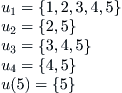
Using the above-mentioned method to Example 1.4 and 1.5, we still have the solutions as shown in Fig. 1.5.
Using Proposition 1.7, when X is a finite set, the directed graph corresponding to (pseudo) semi-order on [X] can easily be defined as follows: 
 , where
  means there exists a directed edge between a and b. The (pseudo) semi-order corresponding to the directed graph is just the quotient structure on [X].
1.5.1.2. Falsity (Truth)-Preserving Principle
The order-preserving ability among different grain-size worlds has an extensive application. For example, the relation among elements of domain X is represented by some semi-order structure. A starting point is regarded as a premise and a goal point  as a conclusion. Whether the directed path from point x to point y exists corresponds to whether conclusion y can be inferred from premise x. If X is complex, introducing a proper partition R to X, then we have [X]. A quotient (pseudo) semi-order
  on [X] can be induced. Due to the following proposition, the original directed path finding from x to y on X is transformed into that from [x] to [y] on [X].
Proposition 1.8
(X,T) is a semi-order set. R is an equivalence relation on X. For , if there exists a directed path from x to y on (X,T), there also exists a directed path from [x] to [y] on [X].
The proposition shows that if the original problem (domain) in hand is too complex, by a proper partition, the original domain is transformed into a coarse one. If there does not exist a solution in the coarse world, then the original problem does not have a solution as well. Since the coarse world is generally simpler than the original one, the problem solving will be simplified.
Note that in Proposition 1.4, even R is incompatible, the order-preserving ability still holds.
From the previous discussion, it is known that an ‘inference’ can be transformed into a spatial search from a premise to a conclusion, i.e., a path-search in a topologic space. And if an original problem  is too complex, then the problem can be transformed into its quotient space
  which is generally simpler than the original one. The order-preserving and the falsity (truth)-preserving ability that we will mention below clarify the main characteristics of the multi-granular world; which provide a theoretical foundation for multi-granular computing (inference).
Theorem 1.4 Falsity-Preserving Principle
If a problem  on quotient space has no solution, then problem
  on its original space has no solution either. In other words, if on has a solution, then on has a solution as well.
Proof:
If problem has a solution, then A and B belong to the same (path) connected set C of . Let be a natural projection. Since p is continuous,  is (path) connected on .
  and
and  belong to the same (path) connected set of . The problem has a solution.
Falsity-preserving ability within a multi-granular world is unconditional but truth preserving is conditional.
Theorem 1.5 Truth-Preserving Principle I
A problem on has a solution, if for  ,
,  is a connected set on X, problem on has a solution.
Proof:
Since problem on has a solution,  and
and  belong to the same connected component C. Letting
  , we prove that D is a connected on X.
Reduction to absurdity: Assume that D is partitioned into the union of mutually disjoint non-empty open close sets  and
and  . For
. For  ,
,  is connected on X, then only belongs to one of and .
  , composes of elements of [X]. There exist
  such that
  . Since
  are open close sets on X and p is a natural projection, are non-empty open close sets on [X]. While
  and
and  are the partition of C, then C is non-connected. This is a contradiction.
Theorem 1.6 Truth-Preserving Principle II
How to make use of the falsity- and truth-preserving principles will be discussed in Chapters 5 and 7.
1.5.1.3. Computational Complexity Analysis
Using the falsity- and truth-preserving principle, the computational cost of the multi-granular computing (or inference) can greatly be reduced. For example, by choosing a proper quotient space and using the falsity-preserving principle, the part of the space without solution can be removed for further consideration so that the computing is accelerated. Similarly, by choosing a proper quotient space and using the truth-preserving principle I, the problem solving on the original space can be simplified to that on its quotient space. In general, the size of the quotient space is much smaller than that of the original one so the computational cost is reduced. Concerning the truth-preserving principle II, assume that n and m are the potentials of  and
and  , respectively. The potential of
  is nm at most. Let
  be the computational complexity. When the problem is solved on directly,
  . If using the truth-preserving principle II, the problem is solved on and , separately, the computational complexity is
  . This is equivalent to reducing the complexity from
  to
to  .
.
Note that  , a topology on
  , is not necessarily an induced quotient topology
  of , generally
  . Namely, is only an element of complete semi-order lattice V but U.
1.5.2. Quotient Structure
In the previous section, we discussed two specific spaces, i.e. topologic and semi-order spaces, the general topologic structure will be shown below.
Definition 1.24
Given a problem space , and has some attribute H, if we introduce a structure [T] into [X] such that p(A) on ([X], [f], [T]) has the same attribute H, then [T] is said to be a quotient structure with attribute H, where is a natural projection.
If (X, T) is a topologic space and ([X], [T]) is its quotient topologic space, [T] is a quotient structure with the connectivity (H) within .
If (X, T) is a semi-order space and its quotient space  defined in Section 1.5.1.1 (2), is a quotient structure with order preserving ability.
When we have natural projection and quotient space  , the operators, concepts, functions, etc. defined on X can formally be removed to easily. For example, assuming
  is a function, define a corresponding function
  on such that
  . Generally, all attributes of g on are not necessarily kept in that of
  on completely. This means that in the coarse-grained world some information might lose due to the abstraction, if the missing attributes are not interested, that does not matter very much. But for the attributes that we needed, they should be preserved by choosing a proper partition.
In conclusion, we know that for different purposes, from a computational object , different quotient sets [X] may be constructed and in the same quotient set different quotient structures [T] may be induced, i.e., choosing a proper granularity. This is the key to multi-granular computing.
Finally, the classification with overlapped components will be discussed in Section 3.4.8.
..................Content has been hidden....................
You can't read the all page of ebook, please click here login for view all page.