5.4. Dimension Reduction Method
The RMG of moving object A among obstacles is usually high-dimensional. The judgment of the connectivity of  is rather difficult when the environment of A is cluttered up with obstacles. Based on the multi-granular computing strategy, we may observe the connectivity of the high-dimensional graph from its quotient space, if the connectivity is preserved in that space. Since the quotient space is simpler than the original one generally, this will make the complexity reduced.
Based on the basic idea above, we present a dimension reduction method for investigating the connectivity of high-dimensional graph. Roughly speaking, if E is a subset in a high-dimensional space  there exists a unique mapping
  such that
  . If f satisfies certain conditions, the connectivity of E can be inferred from the connectivity of the domain of f and
  . This is called a dimension reduction method.
5.4.1. Basic Principle
We now use some topologic terminologies and techniques to show the basic theorems of the dimension reduction method. Readers who are not familiar with the contents are referred to Eisenberg (1974) and Sims (1976).
The mappings discussed in point set topology are usually single-valued. But the mappings concerned here are multi-valued. It is necessary to extend some concepts of topology to the multi-valued mappings.
For simplicity, the spaces addressed here are assumed to be metric spaces.
Definition 5.11
Definition 5.12
If  is semi-continuous at any point of
  , then is semi-continuous on .
Definition 5.13
Definition 5.14
F is a mapping from  and is called a union mapping of
  and
and  .
.
Theorem 5.2
Proof
Assuming that  is not connected, then
  , where
  and
and  are mutually disjoint non-empty open sets. Let
![]()
Since  , is connected and sets and are separated, then either
  or
or  holds. We assume that .
For any  , there exists
  . Let
. Let  . Since is open, is a neighborhood of
  .
.
From the semi-continuity of F, for  there exists a
  such that when
  ,
,  holds. Namely,
  . We have
  . Thus,
  is open.
Similarly,  is also open.
Finally, we show that  must hold. Otherwise, there exists
  , that is, and
  . Since is connected and sets and are separated, we have and . This is in contradiction to
  .
.
Therefore,  , i.e., can be represented by the union of two mutually disjoint non-empty open sets. This is in contradiction to that is connected.
The theorem is proved.
Theorem 5.3
Proof
Let mapping  be
be  .
.
From the definition of the product topology, it is known that given  and a neighborhood
  of
of  , for
, for  , there exists a neighborhood of z such that
  , where
  and
and  .
.
Since is compact is also compact in  . Besides,
  is an open covering of , then there exists a finite number of sub-coverings
  .
.
Let  ,
,  , where
  .
.
Therefore, we have  .
.
Finally, from the semi-continuity of F, for  , there exists a neighborhood
  of
of  such that
  .
.
Letting  , for
, for  we have
![]()
Thus, for we have
![]()
![]()
Namely, G is semi-continuous at . Since is an arbitrary point in , G is semi- continuous on .
On the other hand, since is connected, we have that  is also connected.
From Theorem 5.2, we conclude that  is a connected set in .
Theorem 5.4
For  , E is compact.
  is a mapping corresponding to E, i.e.,
  . Then, F is a semi-continuous mapping from .
Proof
Since is compact, if F is not semi-continuous, there exist  and
and  such that for any n, there has
  such that
  , where
  is a metric function on . Namely,
  and
and  exist.
Let  . Since
  is compact, there exists a sub-sequence (still denoted by
  ) such that
  , i.e.,
  .
.
Since is open and , there exists a positive number  such that
  . Thus, there exists
  when
when  have
have  . This is in contradiction with .
Therefore, F is semi-continuous.
Corollary 5.2
If moving object A is a polyhedron and the obstacles consist of a finite number of convex polyhedrons  , then the rotation mapping
  of A among the obstacles is a semi-continuous mapping, where D is the activity range of A, S is a unit sphere and C is a unit circle.
Proof
From Theorem 5.4, it’s only needed to prove that the RMG corresponding to A is compact.
Assume that  is a RMG corresponding to
  . Since
  and sets
  and
and  are bounded subsets in three-dimensional Euclidian space, from topology, it’s known that in n-dimensional Euclidian space, the necessary and sufficient condition of a compact set is that it’s a bounded closed set. Thus, in order to show the compactness of set , it’s only needed to show that set is closed.
First we made the following agreement. When object only touches obstacles, its state is still regarded as a point in . When object overlaps with obstacles, i.e., they have common inner points, its state is regarded as not belonging to .
In order to show that is closed, it’s only needed to show that the complement  of is open.
For any  , from the above agreement, it’s known that when and obstacle
  (may as well assume that
  ) have common inner points, i.e., there exists
  , where
  is an inner kernel of . Thus, there exists a neighborhood
  of .
of .
Assume that is a fixed point O. Some direction via point is denoted by  . Then
  can be represented by
  . In fact, and correspond the same position of A. The different representations of the same position in A due to the different options of its fixed point and direction.
Let  . Obviously,
  is a neighborhood of
  . Since
  no matter A locates at arbitrary position of , and always have common inner points. In other words, any point in always belong to . Thus, is open, i.e., is closed.
Theorem 5.5
Proof
From Theorem 5.3, we have that  and
and  are connected. Since there exists a such that
  then
then  . From Property 5.3 in Section 5.3, we know that
  is a connected set.
Theorems 5.2–5.5 underlie the basic principle of the dimension reduction method that related to the connectivity structure of a set in a product space. Namely, the connectivity problem of a set , or an image  in the product space , under certain conditions can be transformed to that of considering the connectivity of domain and , respectively. Since
  obviously the dimensions of both and
  are lower than that of . So the dimension is reduced.
Furthermore, if or is also a product space, then a set on or can be regarded as an image of a mapping in an even lower space. By repeatedly using the same principle, a high-dimensional problem can be decomposed into a set of one-or two-dimensional problems.
In the collision-free paths planning, its state space can be regarded as an image of mapping . From Theorem 5.2, the state space can also be regarded as an image of mapping  ,
,  or
or  . Therefore, according to the concrete issue, we can choose state space representations based on different mappings which will bring considerable convenience to path planning.
In fact, the dimension reduction method is one of the specific applications of the truth and falsity preserving principles in quotient space theory.
5.4.2. Characteristic Network
In Section 5.3, we presented a general principle for constructing a characteristic network which represents the connected structure of a set. In this section, we will use the dimension reduction method for constructing the characteristic network.
The Connected Decomposition of a Mapping
In Section 5.3, the concept of the homotopically equivalent class is introduced. We now extend the concept to sets in general product spaces.
Definition 5.15
(1)  and
and  are arcwise connected on X
(2) Assume that  , the image of F on D, has m connected components
  , then
  has just m connected components.
(3) If has m components then  , where
  is a projection. Then, is said to be a homotopically equivalent class of with respect to X, or is a homotopically equivalent class for short.
If has m connected components, denoted by , letting  be a mapping corresponding to
  , then is called the connected decomposition of F with respect to D.
Let's see an example.
Example 5.6
Now,  is decomposed into two homotopically equivalent classes
  and
and  .
.
Graph  has two connected components
  and
and  . Their corresponding mappings are
  and
and  , respectively.
Graph  has one component
  . Its corresponding mapping is
  .
.
Thus,  is the connected decomposition of
  . is called a connected component of on
  .
.
The Construction of Characteristic Networks
The connected decompositions of on are  . Let
. Let
![]()
The construction of a characteristic network is as follows.
(1) For each  , constructing a node
  , we have a set
  of nodes.
(2) For  and
and  , if their corresponding components
  and
and  are neighboring in , i.e., the intersection of their closures is non-empty, then and
  is said to be neighboring.
(3) Linking each pair of neighboring nodes in  with an edge, we have a network
  . It is called a characteristic network corresponding to
  , or a characteristic network corresponding to F.
Proposition 5.6
Note that a  corresponds to a node
  that means
  , where
  is a set of corresponding to node
  .
.
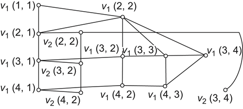
Example 5.7
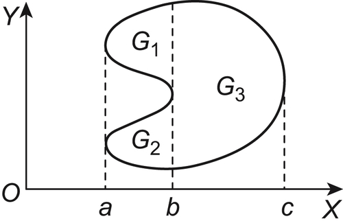
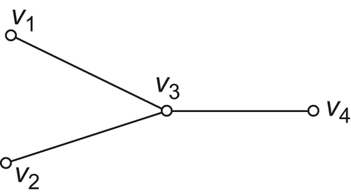
A set as shown in Fig. 5.17 is given. is decomposed into sets  and as shown in Fig. 5.17. Its characteristic network is shown in Fig. 5.18.
Note that to judge the neighboring relationship between and , their closures  and
and  are constructed only on . Since the intersection between their closures is empty, and are not neighboring. However, to judge the neighboring relationship between and , their closures are constructed on
  .
.
Generally, to judge the neighboring relationship between two sets and  , their closures are constructed on
  .
.
Certainly, can also be decomposed into three homotopically equivalent classes  and
and  . And we have a characteristic network as shown in Fig. 5.19.
Where
![]()

Obviously, if is decomposed into the union of maximal sets of homotopically equivalent classes, the number of nodes in the corresponding characteristic network will be minimal.
Finally, we analyze the dimension reduction method from quotient space based granular computing view point.
Now is decomposed into the union  of homotopically equivalent classes. For
  ,
,  , is regarded as a quotient space composed by equivalence classes and is denoted by
  . Each element on is a connected set on . The problem solving in space can be transformed into the corresponding problem solving on since these two spaces have the truth preserving property.
If regarding  as an equivalence class, we have a quotient space
  . It still has the truth preserving property; so the original problem can also be transformed into a corresponding problem in space. Moreover, the problem in can be further transformed into a corresponding problem in a characteristic network. Thus, the characteristic network method of path planning is an application of quotient space theory.
Collision-Free Paths Planning
Assume that a moving object A is a polyhedron with a finite number of vertices and the obstacles  are convex polyhedrons with a finite number of vertices.
Let  be the rotation mapping of A with respect to obstacle
  , i.e.,
  is an intersection mapping of
  .
.
Let  be the connected decompositions of .
According to the preceding procedure, we may have a characteristic network  and the following proposition.
Proposition 5.7
Given an initial state  and a goal state , if
  and
and  then object A can move from to without collision, if and only if there exists a connected path from
  to
to  on .
on .
An Example
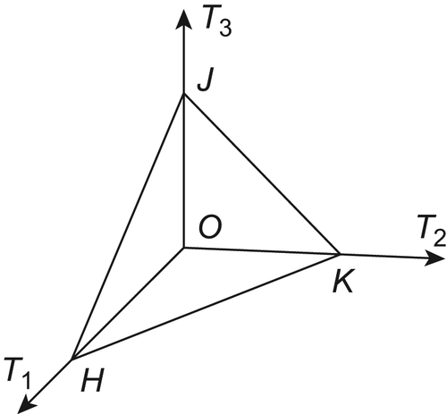
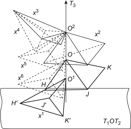
Assume that the moving object A is a tetrahedron (Fig. 5.20). The initial coordinates of its four vertices are  and
and  . Plane
  is an obstacle.
We next analyze the topologic structure of the RMG of the tetrahedron A due to obstacle .
The state of a rigid object A can be defined by the coordinates of any non-colinear three points on A, e.g., and
and  . The coordinate of the point O is
  . Its range is the upper half space, i.e.,
  and is denoted by D. If point O is fixed, the range of H is a unit sphere S with O as its center and
  as its radius, i.e.,
  . If points O and H are fixed, the range of K is a unit circle C with O as its center. And the circle is on the plane perpendicular to line OH via K, i.e.,
  . Generally, D, S and C are represented by rectangular, sphere and polar coordinate systems, respectively.
The RMG of the moving object A is a subset of space  (six-dimensional), i.e., the state space of A.
From Section 5.3, we know that the RMG of A can be regarded as an image of mapping  . Since the obstacle is a plane, the state space of A remains unchanged for coordinates
  and horizontal angle
  on S; so it’s only related to three parameters, i.e.,
  and
and  .
.
Now, we discuss its characteristic network.
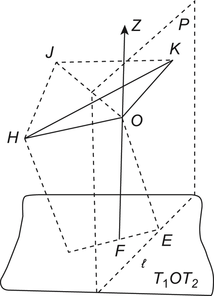
(1) Fix  and
and  , to find
  .
.
As shown in Fig. 5.21, through K we compose a plane P perpendicular to line OH. l is an intersecting line between planes P and . Through line OH we compose a plane perpendicular to . OE is an intersecting line between the composed plane and P.
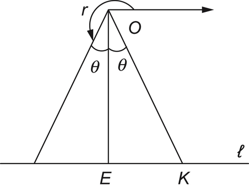
As shown in Fig. 5.22, in plane P, the line through point O and parallel to l is used as a reference axis. The position of point K can be represented by the angle  related to the axis.
Obviously, if  , the range of point K is the entire unit circle and is denoted by
  .
.
Similarly, the range of point J is also the same circle when it is transformed to a constraint of point K, i.e.,  .
.
Thus,  , i.e., has only one component.
When  ,
,  and
and  , where
  .
.
The second component will disappear when  , i.e.,
  . Therefore, when
  , the mapping has two components. When
  , it has only one component.
(2) The relationship between and OH
In (1) we discuss the relation between and OE. Actually, the length of OE depends on the position of OH, i.e., coordinate and .
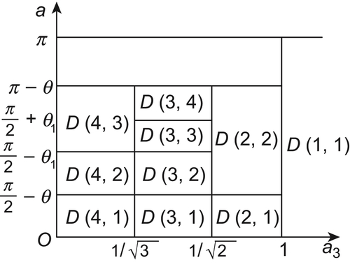
Assume that the coordinate of the point O is . The coordinate is divided into four intervals: (i)  , (ii)
  , (iii)
  , (iv)
  . Each interval of is further divided into several sub-intervals based on the value of .
The partition of and is shown below (Fig. 5.23), where  ={the i-th interval of , the j-th interval of }.
To show the procedure of calculating , we take interval as an example.
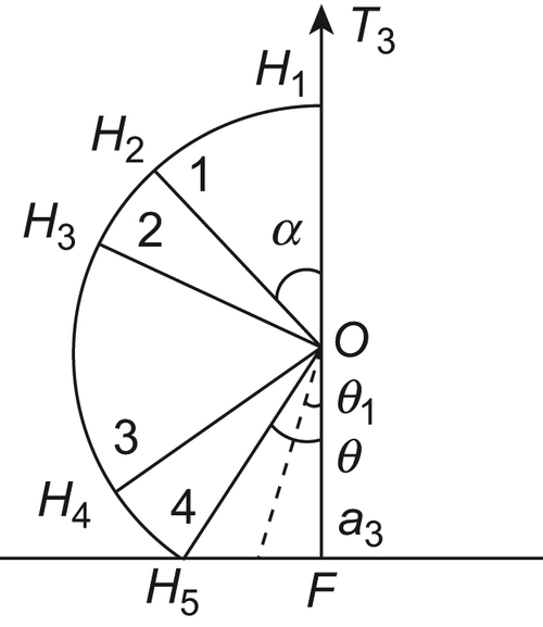
Fixing point O, through O we compose a line  parallel to
  -axis (Fig. 5.24). The position of OH is defined by angle . Then, angle is divided into four intervals.
 . When , the range of point H on S is
  , where
  and
and  .
.
![]()
We can write that
When  ,
,  since .
When  has two components since
  .
.
When  , has one component since
  .
.
When  , has two components since .
Let be the k-th component of on . If is connected, then it is denoted by  .
.
Let  , i.e.,
  is the image of
  .
.
Similarly, we have the following results.
When , has one component, i.e.,  ,
,  .
.
When ,
When
(3) Characteristic network
Each corresponds to a node  . We have a set V of nodes.
Nodes and  of V are neighboring if their corresponding
  , are neighboring in the state space.
Linking any pair of neighboring nodes by an edge, we obtain a characteristic network (Fig. 5.25).
(4) Find collision-free paths
And given a goal state  , where
![]()
![]()
![]()
![]()
Then,
![]()
From the characteristic network , we have a collision-free path of A.
Note that only one parameter changes in each step. For example, from state  , only the coordinate changes from
  . The range of each parameter is indicated in the brackets.
The moving process of A is shown in Fig. 5.26.
(5) Conclusions
The configuration space representation and the like are usually used in both geometric and topologic approaches to motion planning. The main difference is that in the geometric model the geometric structure of  is investigated, while in the topologic model only the topologic structure is concerned.
Taking the ‘piano-mover’ problem as an example, by the subdivision algorithm presented in Brooks and Lozano-Perez (1982), the real is divided. Even though the connectivity network constructed consists of 2138 arcs linking 1063 nodes, it is still an approximation of the real . But in the topologic algorithm (see Section 5.5 for the details), the characteristic network constructed only consists of 23 nodes linked by 32 arcs, however, it is homotopically equivalent to the real . Therefore, from the connectivity point of view, the topologic model is precise (Zhang et al., 1990a).
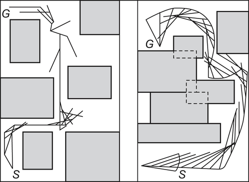
Since in topologic model, the motion proceeds in the coarse-grained world the computational complexity may be reduced under certain conditions. In 1980s we implemented the ‘piano-mover’ problem by topologic method on PDP 11/23 machine. The program is written by FORTRAN 4 and takes about dozens of seconds CPU time for implementation. More results will be given in Section 5.5. We also implemented dozens of experiments on ALR-386/II machine for a 2D rod moving among obstacles using programing language PASCAL and take less than 15 seconds time for implementation. One of the examples is shown in Fig. 5.27.
..................Content has been hidden....................
You can't read the all page of ebook, please click here login for view all page.