5.5 Applications

Search in book...
Toggle Font Controls
Create new playlist

Name your new playlist

Playlist description (optional)
Sign In

Email address

Password

Forgot Password?

or

Continue with Facebook

Continue with Google
Sign Up

Full Name

Email address

Confirm Email Address

Password

or

Continue with Facebook

Continue with Google

5.5. Applications

In this section, the theory and technique presented in the preceding sections will be applied to two motion planning problems. One is the planning for a planar rod moving among obstacles. The other is the planning for a multi-joint arm (Zhang and Zhang, 1982a, 1982b, 1988b, 1990a).

Figure 5.28 r-Growing Boundaries

The main point for using the theory to a real motion planning problem is how to decompose the domain into homotopically equivalent classes. There are three kinds of boundaries which are used for the decomposition. Namely, the original boundaries of the obstacles, the r-growing boundaries of the obstacles, and some specific curves called the disappearance curves arising in the regions cluttered up with the obstacles.

5.5.1. The Collision-Free Paths Planning for a Planar Rod

Assume that the length of rod A is r. The obstacles are assumed to be composed of a finite number of convex polygons. One of the end points of rod A is regarded as a fixed point O. The activity range of point O is a region in a two-dimensional plane. The rod itself is regarded as a reference axis OT. The activity range of OT-axis is its orientation angle.

The state space of A is X. We regard X as an image of mapping

, where D is the activity range of point O and C is a unit circle.

The Homotopically Equivalent Decomposition of Domain D

Definition 5.16

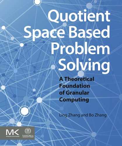
Assume that the length of rod A is r. We define the r-growing boundaries of obstacles as follows.

As shown in Fig. 5.28, B is an obstacle. We construct new lines parallel to and at a distance r from each edge of B, and draw arcs with each vertex of B as its center and r as its radius which are tangent to the new lines. The boundary composed of these new lines and arcs is called the r-growing boundary of obstacle B (Fig. 5.28).

Definition 5.17

and

are two obstacles (Fig. 5.29).

is a segment of r-growing boundary of B₂.

is an edge of

. If

is inside of

in part then we said that

and

compose a ‘lane’.

Figure 5.29 A ‘Lane’

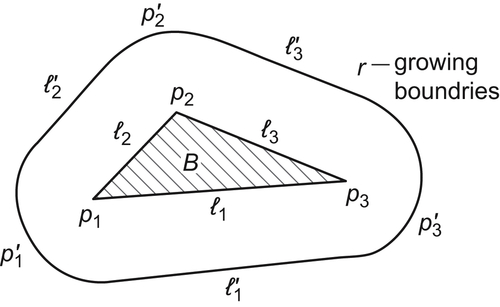
As shown in Fig. 5.29, at point

there exist the feasible orientations of OT along the direction of the lane, but at point

there does not have any feasible orientation since it is blocked by obstacle

. Under the edge

, there is an area where rod A does not have any feasible orientation along the direction of the lane. It is called a shaded area. The boundary of the shaded area can be computed as follows.

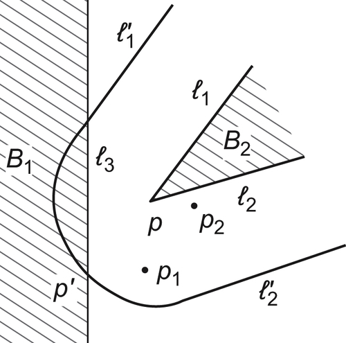
As shown in Fig. 5.30, we regard the boundary

-axis, the line perpendicular to

through point p as

-axis and the angle

formed by OT and

-axis as a parameter. The equations of the boundary S of the shaded area are shown below.

where,

is the coordinate of the points on S,

is the angle formed by

and

-axis, and a is the distance between point p and boundary

The boundary S is called a disappearance curve, since some orientation components will disappear when the rod going across the boundary.

Figure 5.30 A Shaded Area

The Decomposition of the Homotopically Equivalent Classes

The original boundaries and r-growing boundaries of obstacles and the disappearance curves will divide domain D into several connected regions denoted by

We will show that

is a homotopically equivalent class, where set

is the inner kernel of D.

Let

be the rotation mapping of A. Given

, it is easy to find

or each component of

Given

, using x as center and r as radius, we draw a circle C counter clockwise. C is divided into several arcs by the central projections of obstacles from x on C. Then each arc corresponds to a component of

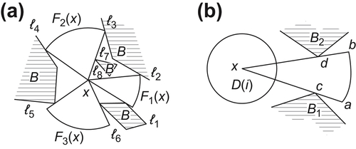
As shown in Fig. 5.31(a),

is decomposed into three components

and

. As shown in Fig. 5.31(b), each arc

corresponds to a component

. c(d) is the point of intersection between obstacle B₁ (B₂) and radius ax(bx). Points c and d are called intersection points of component

on obstacles or simply the intersection points of

. As shown in Fig. 5.31(a), component

can be represented by (1,2) or (8,2), where numbers 1, 2 and 8 indicate the numbers of edges l₁, l₂ and l₈ of obstacles, respectively. And the intersection points of

locate in edges l₁, l₂ and l₈. Similarly,

is denoted by (3,4), (7,4) or (9,4), etc. By this notation a component may have different representations but they should be regarded as being the same component.

Definition 5.18

A mapping

, where

and

are metric spaces. If

, for

such that when

, we have

where

Figure 5.31 The Connected Decomposition of F

Then F is said to be continuous at

. If

, F is continuous, then F is said to be continuous on X.

Proposition 5.8

The

defined above is a homotopically equivalent class with respect to the rotation mapping F of rod OT, i.e., F is continuous on

Proof

is a connected component of

. As shown in Fig. 5.31(b), there is no obstacle inside the sector

. But there is at least an intersecting point between edge

and the obstacles. There doesn't lose generality in assuming that only one such point exists at each edge, i.e.,

, where

and

are obstacles.

If arc

is degraded into a point, then x is a point at the boundary of some shaded area or a is a concave vertex of some obstacle. This is a contradiction.

is a vertex of some obstacle, then

. Otherwise, x belongs to a vertex of some r-growing boundary. This is a contradiction, too.

Thus, the length of

is assumed to be positive, a and b are not vertices of obstacles and sector

is at a positive distance from the rest of obstacles except

and

. Therefore, given

for

, we construct every rounds with y as its center and r (the length of the rod) as its radius. The sectors, parts of the rounds that locate between obstacles

and

, are non-empty. And the sector is at a distance from the rest of obstacles except

and

. Thus, the arc corresponding to the sector is a connected component of

denoted by

satisfying

Namely,

is continuous at x.

For each component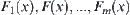

, we conduct the same analysis and obtain that when x changes from

continuously, each component

will change from

continuously, respectively. Thus,

is a homotopically equivalent class.

The Construction of Characteristic Network

(1) Domain

is divided into several connected regions by the original boundaries, r-growing boundaries of obstacles, and the boundaries of the shaded areas. The connected regions are denoted by

(2) To find the components of

on each region

, it only needs to find the components of

for any

. Then, we have a set

of components.

Where,

denotes the image of component

, and component

represents the component lied between edges

and

(3) Node

is constructed with respect to each

. We have a set V of nodes.

Assume that

and

are neighboring. According to different forms of their common edge, there are four different linking rules.

(a)

is their common edge, where

is the r-growing boundary of edge

. Assume that

is on the inside of

, i.e.,

is located between

and

. Then

and

are linked with

(b)

is their common edge, where

is a r-growing boundary of vertex p.

is on the inside of

. Then

and

are linked with

If p is a concave vertex, i.e., the angle corresponding to vertex p is greater than 180, then

is not linked with any

and

is on the inside of s, then

is not linked with any

(d)

is linked with

, i.e., the components with the same name in

and

Based on the preceding rules, linking the nodes in the set V, we have a network

is the characteristic network corresponding to the rod A.

Examples

Example 5.8

The obstacles are shown in Fig. 5.32. Find the characteristic network of rod OT.

Solution

D is divided into 13 regions shown in Fig. 5.32. Taking the number of each region

as the horizontal ordinate, and the number (double index) of each component as the vertical ordinate, if

exists, and then we draw a node

in the point where the horizontal ordinate is i and the vertical ordinate is

. Then, we have the characteristic network as shown in Fig. 5.33.

Figure 5.32 One-Dimensional Rod

Figure 5.33 Characteristic Network

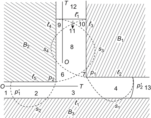
, the boundary of shaded area, is the common edge of

and

, then

is not linked with any point in

, according to the rule.

is the common edge of

and

, where the two included sides of

are

and

, then

and

are linked with

, according to the rule. But

is on the inside of

, component

disappears. Finally,

is connected to

. Moreover,

is connected to

with the same name.

The same rules are applied to other components. Finally, the characteristic network we obtained is shown in Fig. 5.33.

From Fig. 5.33, we can see that the characteristic network consists of three disconnected sub-networks. This implies that rod OT can't move from a state to an arbitrary state, e.g., from state

rod OT can't move to state

, since there is no connected path from node

to node

in the network (Fig. 5.33).

Example 5.9

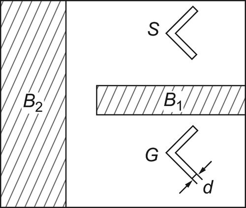
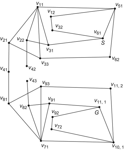
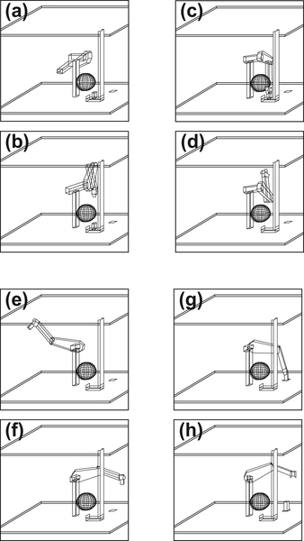
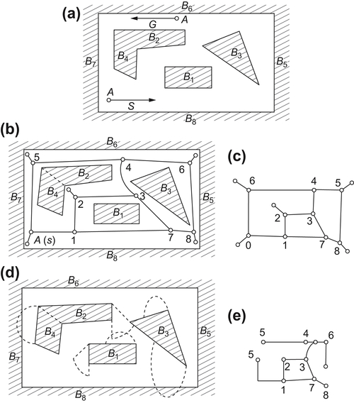
The ‘Piano Mover’ problem is that given a ‘piano’ A and the obstacles as shown in Fig. 5.34, find a path from the initial position S to the goal position G.

For simplicity, piano A is shrunk to a broken-line while the boundaries of obstacles B₁ and B₂ are enlarged by the size 1/2 d, where d is the width of the piano A.

Domain D, the XOY plane, is divided into 10 regions as shown in Fig. 5.35.

Its characteristic network is shown in Fig. 5.36.

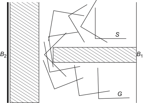
The final result implemented by computers is shown in Fig. 5.37.

5.5.2. Motion Planning for a Multi-Joint Arm

Multi-Joint Arm

A multi-joint arm R consists of

axis and m arms

, as shown in Fig. 5.38.

Figure 5.34 Piano Mover

Figure 5.35 The Partition of Domain D

Figure 5.36 Characteristic Network

Figure 5.37 The Result of Piano Mover

Figure 5.38 A Multi-Joint Arm

The rotation angle about

is denoted by

. The rotation angle of each arm

around

is represented by

. The length of arm L_i is

. The obstacles are assumed to be composed by a finite number of convex polyhedrons.

The problem is to find a collision-free path for the arm from the initial position to the goal position.

Rotation Mapping

Assume that

is the state space of a moving object and

is its rotation mapping. X is assumed to be compact. In fact, when D and Y are the subsets of Euclidean space, so long as X is bounded and closed X is compact.

are the homotopically equivalent classes of D.

are the connected decompositions of F.

Let

be the image of component

and

are neighboring if and only if

, where

is the closure of D.

Some properties of the image of the rotation mapping are given below.

Proposition 5.9

F is a mapping from

is the image of F. Assume that

is compact and

has a finite number of connected components. Let

be a homotopically equivalent class of F.

is a connected component of F on

. Then we have that

is semi-continuous.

Proof

Let

and

be the closure of

. Let

be a mapping corresponding to

. Since

is a closed subset of the compact set

is also compact. From Theorem 5.4, we have that

is semi-continuous.

Again,

is a connected component of F on

. So

is a closed set on

, i.e.,

. We have

Namely,

, have

. We conclude that

is semi- continuous.

Definition 5.19

is compact,

and

, are two homotopically equivalent classes. Let

be a connected component of

is a mapping corresponding to

. If

and

are neighboring and

, we have

, then

and

are called regular neighboring, where

is the closure of D.

is the image of F on D.

Corollary 5.3

and

are regular neighboring, by letting

be the union mapping of

and

, then

is semi-continuous.

Proposition 5.10

Under the same assumption of Corollary 5.3, by letting

be a mapping corresponding to

, and

be a connected subset, then

is a connected set.

Proof

From Corollary 5.3 and dimension reduction principle, it now only needs to prove that

is connected.

From the definition of the homotopically equivalent class, it easy to show that

is connected. We now show that

is connected.

By reduction to absurdity, assume that for

is not connected. Since

is compact, there exists

such that

, where

and

are non-empty,

, and

Since

is semi-continuous, there exists

such that

We obtain

However,

and

are separated sets. Again, it is known that

is connected.

is connected and

is semi-continuous. Thus,

is a connected set, so it can only belong to either

Assume

, i.e.,

, we have

. Hence,

. This is in contradiction with the assumption. We have that

is connected.

Similarly,

is connected.

, we have

. Therefore,

is connected.

Similarly,

, we have

. Therefore,

is connected as well.

When

, since

and

, we have that

is connected.

Finally, since

is semi-continuous and A is a connected set, from the dimension reduction theorem, we conclude that

is connected.

From the proposition, we can see that if two images

and

are regular neighboring, then the problem of considering the connectivity of

can be transformed into that of the connectivity of

. If

and

are regular neighboring, then the connectivity of

can also be transformed into that of still lower dimensional space. This is just the principle of dimension reduction.

Characteristic Network

(1)

is the end point of a robot arm. All possible positions of

among obstacles are called the domain of

denoted by

(2)

is a mapping,

denotes all possible positions of the end point

of arm

among obstacles, when the other end point

is located at x.

In fact,

is the rotation mapping of x. The only difference is that

is represented by the positions of

rather that the rotation angle

is the rotation mapping of the robot arm on

can be defined by

recursively.

Let

. i.e.,

is a point

have been defined, then we define

as follows.

(3) The connected decomposition mapping

is divided into several homotopically equivalent and connected regions

Assume that the connected decomposition sub-mapping

The image of

denoted by

. Moreover, let each pair

of neighboring images be regular neighboring.

When the moving object is a polyhedron and the obstacles consist of a finite number of polyhedrons, the homotopically equivalent set decomposition of D and the connected decomposition of F will make the neighboring images

become regular neighboring.

(4) Characteristic network of arm

Using the same method presented in Section 5.4.2, we have the characteristic network of

denoted by

The Construction of Characteristic Network

Assume that

are characteristic networks corresponding to

, respectively.

We compose a product set

Let

and

Assuming that

have been obtained, we define

where,

is a connected component with respect to point

is a domain corresponding to

Definition 5.20

Given

, if

then v is a node of characteristic network

, i.e., we have a set V of nodes,

Definition 5.21

Given

and

, where

and

are called neighboring if and only if

and

are neighboring in

Linking each pair of neighboring nodes in V with a line, we have a network

, or N for short. It is called a characteristic network of a multi-joint arm R.

Next, an example of motion planning for a 3D manipulator is shown below.

Example 5.10

A manipulator and its environment are shown in Fig. 5.39. The initial and final configurations are shown in Fig. 5.39(a) and Fig. 5.39(b), respectively. Based on the dimension reduction principle, we have developed a path planning program for a three-joint arm among the obstacles composed by a finite number of polyhedrons and spheres, using C language. The program has been implemented on SUN 3/260 workstation. One of the results is shown in Fig. 5.39. The CPU time for solving the problem is 5–15 seconds in average.

5.5.3. The Applications of Multi-Granular Computing

In motion planning for a multi-joint arm, the concept of multi-granular computing has been used for solving several problems.

Figure 5.39 Motion Planning of a 3D Manipulator

In the construction of characteristic network

, we regard

as a subset of the product set

. To find a connected path from the initial state

to the final state

, a connected path from

is found first, then a connected path from

is found such that the path merged from these two is a connected path from

in the product space

. The process continues until a connected path from

is found, or the existence of collision-free paths is disproved.

This is a typical application based on multi-granular computing. Since

is the projection of

, however, ‘projection’ is one of the multi-granular computing approaches as mentioned in the above chapters.

The dimension reduction method itself is an application based on the multi-granular computing technique as well. The original problem of finding the connected structure of a set

is transformed to that of finding the connected structure of

and

, where F is a mapping corresponding to E. Since

and

both are the projections of E on different spaces, the multi-granular computing technique underlies the dimension reduction method.

In the proceeding applications, the multi-granular computing technique is used mainly through the projection method. Next, other methods are discussed.

The Hierarchical Planning of a Multi-Joint Arm

R is a multi-joint planar manipulator composed of m arms. To find a collision-free path from state

to state

among the obstacles, the motion planning can be made in the following way. First, a primary plan is found by some heuristic knowledge. Then, the plan is refined.

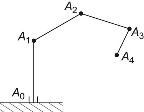
As shown in Fig. 5.40, R is a multi-joint arm moving among the planar environment consisting of obstacles

and

are the initial and final positions of R, respectively.

To plan the primary path, we compose a loop from

along the direction

. i.e.,

, then from

, finally from

along the direction

back to

. i.e.,

. If there is no obstacle inside the loop, then the manipulator can ‘move’ from

directly without collision. Therefore, in this case only a limited portion of N(r) needs searching in order to find the path.

If there are obstacles inside the loop, as shown in Fig. 5.40, obstacles

and

are inside the loop. Then, to move the manipulator around the obstacles, the initial positions of end points

of each arm must first move from

to the left of obstacle

. In other words, from a high abstraction level, we first estimate the primary moving path of R by ignoring the interconnection between arms. Namely, the end point

of arm 7 first moves along the direction

from

to the left of obstacle

, i.e., point

, then moves to

, finally moves to

along the direction

End points

move in a similar way.

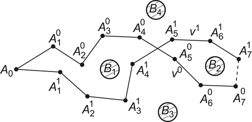
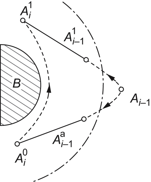
Figure 5.40 Motion Planning of a Multi-Joint Arm

Figure 5.41 A Rod Moves Around an Obstacle

If the end point

of arm

needs to move from one side of obstacle B to the other (Fig. 5.41), then the end point A_i−1 must move from the inside of the r-growing boundary to the outside of the boundary and then back to the inside of B. Namely, the moving trajectory of point

is constrained by the trajectory of point

By using these kinds of heuristic information, the primary moving path of R can be worked out. Then under the guidance of the primary path, a final path can be found.

In three-dimensional case, some proper sections can be used. The two-dimensional characteristic networks can be constructed on these sections. By using the neighboring relationship between the nodes on the neighboring two-dimensional characteristic networks, the characteristic network of the three-dimensional case can be constructed.

As shown in Fig. 5.42(a), we construct the sections

. Let

be the two-dimensional characteristic network on section

is a connected network,

is said to be a connected section. Therefore, when net

is a connected one, section

does not intersect with any obstacle.

Assume that

and

are two neighboring sections of

. If one of

and

is a connected section, then when finding a connected path from state

, we first transform the state

to a state

, then on

move state

to state

. Finally,

is transformed to state

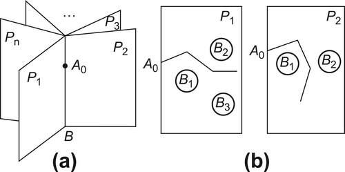
Figure 5.42 Three-Dimensional Characteristic Network

Thus, the three-dimensional case can be handled in the similar way as in the two- dimensional case.

5.5.4. The Estimation of the Computational Complexity

Schwartz and Shatic (1983a) presented a topologic algorithm for two-dimensional path planning. Its computational complexity is

, where n is the number of edges of polygonal obstacles. Schwartz and Shatic (1983b) also presented a topologic algorithm for solving ‘piano-mover’. Its computational complexity is

, where n is the number of obstacles and d is the degree of freedom of moving object.

Reif (1979) and Reif and Sharir (1985) presented a revised algorithm. Its complexity is

, and proved that the general ‘piano-mover’ is a PSPACE-hard problem, i.e., NP-hard problem at least.

In a word, the complexity of collision-free paths planning increases with d exponentially even though by using topologic approaches.

Next, we estimate the complexity of the dimension reduction method by taking motion planning for a planar rod as an example.

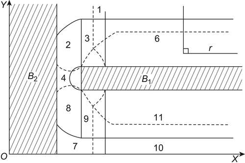
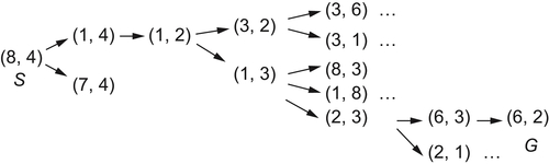
Fig. 5.42(a) shows a rod AT and its environment. When the end point A of rod AT moves from the initial state

, there are three possible moving directions, i.e.,

and

, or (8, 4), (4, 7) and (7, 8) for short, as shown in Fig. 5.42(b). There is no path along the direction (7, 8). Along the direction (8, 4), from point 1 there are two possible moving direction (8, 1) and (1, 4). Along direction (1, 4), from point 2 there also exist two possible moving directions (1, 2) and (2, 4). But direction (2, 4) is a blind alley, etc. We finally have a network shown in Fig. 5.42 (c). It is called a characteristic network of point A denoted by

Network

represents the connected structure of the domain of point A. Each edge

represents an area surrounded by obstacles

and

Based on network

, the movement of rod AT among obstacles can be planned.

Although point A can move freely along each edge of

, rod AT may not. For example, when AT moves from point 1 to 3 through point 2, i.e., turns from direction

to direction

, if we consider the entire rod movement, the movement may not be possible at the intersecting point. Therefore, we must consider the movement at each intersecting point.

Figure 5.43 Path Planning of a Planar Rod

Whether rod AT can turn from one direction to the other may be judged by finding the boundary of the shaded area, presented in the above sections. In the example, the boundaries of each shaded area are shown in Fig. 5.43(d) by the dotted lines.

From Fig. 5.43(d), we can see that turning from direction (4, 7) to (2, 6), from (8, 3) to (5, 3), or from (3, 2) to (6, 2) is impossible. The others are possible. The characteristic network is shown in Fig. 5.43(e).

Given the initial state corresponding to direction (8,4) and goal state corresponding to direction (6,2), we now plan a collision-free path. From (8,4) we search the collision-free paths as shown below.

Finally, we have a collision-free path from S to G (Fig. 5.44):

Figure 5.44 A Collision-Free Path From S to G

Next, we estimate its computational complexity.

Assume there are n convex polygons. By using the concept of dual network and the Euler formula concerning the relationship between points and edges of a planar network, it can be proved that the number of edges in network

is less than or equal to cn, where c is a constant.

Each edge in

represents a direction

, or a ‘channel’ surrounded by obstacles

and

. Strictly speaking, if

and

are r-growing areas of obstacles

and

, respectively, then

is the channel surrounded by

and

To make the turn from the channel

to channel

possible, the necessary condition is that

must intersect the r-growing area of

, i.e., the channel corresponding to edge

intersects

, where

is an edge of N (A),

is the r-growing boundary of

. If the complexity of each judgment is regarded as 1, we have the following proposition.

Proposition 5.12

If the environment consists of n convex polygons, the computational complexity for planning the motion of two-dimensional moving rod is

, if using the above hierarchical planning method.

Certainly, this is just a rough estimation. It is shown that the multi-granular computing strategy has a potential in reducing the computational complexity.

..................Content has been hidden....................

You can't read the all page of ebook, please click here login for view all page.

Table of Contents for 5.5 Applications

Create new playlist

Sign In

Sign Up

5.5. Applications

5.5.1. The Collision-Free Paths Planning for a Planar Rod

The Homotopically Equivalent Decomposition of Domain D

Definition 5.16

Definition 5.17

The Decomposition of the Homotopically Equivalent Classes

Definition 5.18

Proposition 5.8

Proof

The Construction of Characteristic Network

Examples

Example 5.8

Solution

Example 5.9

5.5.2. Motion Planning for a Multi-Joint Arm

Multi-Joint Arm

Rotation Mapping

Proposition 5.9

Proof

Definition 5.19

Corollary 5.3

Proposition 5.10

Proof

Characteristic Network

The Construction of Characteristic Network

Definition 5.20

Definition 5.21

Example 5.10

5.5.3. The Applications of Multi-Granular Computing

The Hierarchical Planning of a Multi-Joint Arm

5.5.4. The Estimation of the Computational Complexity

Proposition 5.12

Table of Contents for
5.5 Applications