
CHAPTER 6
Pricing and Hedging a Swap with Eurodollar Futures
Interest rate swaps make up the lion’s share of the over-the-counter interest rate derivatives market. They are extremely useful for both hedging and trading, are used extensively in corporate funding programs, and are rapidly becoming the core of fixed-income markets throughout the world. The market for interest rate swaps really began to open up in the early 1980s and quickly evolved to the point where most interest rate swaps use LIBOR as the basic reference rate.
The swap market is, in some sense, the end user or retail market for interest rate derivatives, while the Eurodollar futures market is the wholesale market where swap dealers get the raw material for pricing and hedging swaps. The purpose of this chapter is to provide a rudimentary introduction to fixed/floating interest rate swaps and to the relationship between swaps and Eurodollar futures. In this chapter, you will learn how to:
• Determine the size and timing of cash flows on a swap
• Price and hedge a swap using the cash flow method
• Price and hedge a swap using the hypothetical securities method
• Measure convexity differences between forward and futures rates
• Relate a swap yield curve to forward (futures) and zero-coupon yield curves
FIXED/FLOATING INTEREST RATE SWAPS
An interest rate swap is an agreement under which the two counterparties agree to exchange cash flows whose values are determined by the notional size of the swap and by the values of two interest rates. These two interest rates can be whatever rates the contracting parties choose. For example, swap counterparties could exchange cash flows based on commercial paper and Treasury bill rates. The most common swaps, however, are fixed/floating swaps in which the reference rate for the floating side is 3-month LIBOR. In such a swap, one counterparty agrees to receive payments based on a fixed rate that is established when the swap is transacted and to make payments based on a floating or variable rate that is set equal to 3-month LIBOR at key rate setting dates. The other counterparty does just the opposite.
To price or hedge an interest rate swap, you need to be able to determine the size and timing of all cash flows. To do this, you need to know:
• Notional principal amount
• Cash flows in arrears
• Periodicity
• Spot and forward-starting swaps
• Day-count conventions and swap yields
Notional Principal Amount
In principle, the cash flows on the interest rate swap could be replicated by borrowing and lending in the cash market. For example, the cash flows on the fixed/floating swap could be replicated by borrowing short term (say every 3 months) and lending long term (for the life of the swap). If you were replicating the cash flows on a $100 million swap, you would actually borrow $100 million and turn right around and lend $100 million. Also, when the term of the swap is over, you would use the principal value of your asset to pay off the principal value of your liability.
With an interest rate swap, these principal amounts never change hands, so the opening and closing transactions are eliminated. Rather, a swap has what is known as a notional principal amount, which is used only to calculate hypothetical interest payments. For example, on a $100 million swap, you would apply the fixed and floating interest rates to $100 million. The resulting hypothetical interest payments are the swap’s cash flows.
One consequence of this arrangement is that credit exposure in a swap is less than it is in the cash market. Rather than having to worry about the $100 million that someone owes you on your asset, you need worry only about the net present value of the swap, and then only if the net present value is positive and the other person owes you.
Cash Flows in Arrears
With most interest rate swaps, the hypothetical interest payments are paid and received just as they would be on real assets and liabilities—at the end of the interest calculation period. If you were to borrow money for 3 months, you would pay the interest on the loan at the end of the 3 months. And so it is with a swap. Cash flows occur at the end of the interest calculation period.
Periodicity
Fixed and floating cash flows can be done with any periodicity the two counterparties choose. The payments could be made monthly, quarterly, semiannually, or annually. The fixed and floating payments might have the same periodicity, in which case the cash flows are netted, or different periodicity. The floating rate reset dates have their own periodicity, which may or may not match the periodicity of the floating cash flows.
What constitutes the standard mix of fixed and floating payments varies over time, but at this writing, a very common mix is semiannual floating and fixed payments, with the floating rate tied to 3-month LIBOR compounded or to 6-month LIBOR.
Spot and Forward-Starting Swaps
With a spot swap, the initial net cash flow is defined when the trade is executed. For example, if you do a fixed/floating swap that starts today, you would determine both the fixed rate that will be used throughout the swap’s entire life as well as the initial “floating” rate. As a result, you know when the swap is transacted exactly how much cash will change hands at the first cash flow date.
In contrast, a swap can start on a forward date. In this case, you might determine the fixed rate today, when the trade is done, and wait until the forward-starting date to determine the first of the floating rates. A common version of a forward-starting swap is an “IMM” swap, whose rate setting dates correspond exactly to the expiration dates for Eurodollar futures and whose cash flow dates correspond to futures value dates. By design, these swaps are especially easy to price and hedge because there are no date mismatches with the Eurodollar futures market.
Day-Count Conventions and Swap Yields
You also have your choice of day-count conventions for both legs of the swap. The most common would be an Actual/360 money market convention for the floating side and a 30/360 corporate convention for the fixed side. In practice, however, you can choose from:
• Actual/365 or Actual/Actual
• Actual/365 (Fixed)
• Actual/360
• 30/360 or Bond Basis
• 30E/360 or Eurobond Basis
for either the floating or the fixed side, and you can choose a different method for each side.
Swap yields describe the fixed side of the swap. In the dollar market, the usual convention is corporate—that is, semiannual 30/360—although the swap yield often is quoted in the same terms as the thing it is hedging. Therefore, if the swap is hedging a Treasury, its yield would be quoted using Treasury conventions. If it is hedging a LIBOR-based loan, it might be quoted in money market terms.
In keeping with this, swap yields in other markets (e.g., Europe, the United Kingdom, and Canada) tend to be quoted using those markets’ conventions.
SWAP BASICS:1 AN IMM SWAP
Diagram the cash flows for the following 1-year fixed/floating IMM swap:
Notional amount = $100 million
Trade date = June 17, 2002
Maturity date = June 18, 2003
Fixed side
Fixed rate = 2.41%
Payment dates = Eurodollar futures value dates
Day-count convention = Actual/360
Floating side
Reset dates = Eurodollar futures expiration dates
Payment dates = Eurodollar futures value dates
Day-count convention = Actual/360
Floating rate = 3-month LIBOR
Spread over floating reference rate = 0 bp
Floating rate for initial calculation = 1.8788%
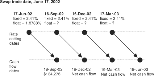
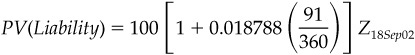
For this IMM swap, the floating rate is reset on Eurodollar futures expiration dates. Payment occurs three months after the rate has been set. The first floating rate, for example, is set on the trade date, June 17. The actual cash flow occurs on September 18, the next futures value date. The swap payment is calculated by netting the fixed and floating rate payments:
![]()
![]()
This first net cash flow of $134,276 is paid to the counterparty that receives fixed and pays floating. The remaining net cash flows are unknown at the time of the trade.
APPROACHES TO PRICING AND HEDGING INTEREST RATE SWAPS
The net cash flows on a fixed/floating swap are designed to mimic exactly the net cash flows that would be produced by combining fixed and floating rate assets and liabilities. For example, the person who receives fixed and pays floating on an interest rate swap could achieve the same thing by borrowing money at a variable rate and lending or investing the entire amount at a fixed rate. In such a transaction, the opening cash flows (i.e., the principal amounts) would offset one another exactly, so the initial net cash flow would be zero. Thereafter, net cash flows would reflect the values of the fixed and variable interest rates. And at the final maturity of the fixed rate asset, the principal amount would be used to pay off the principal amount on the floating rate loan.
With this in mind, you can tackle the problems of pricing and hedging a swap in either of two ways, both of which take you to the same answers.
Cash Flow Approach
With an interest rate swap, the principal amounts do not change hands—only the hypothetical interest payments. Because the initial net cash flow in the hypothetical trade described above is zero, you can solve the problem of pricing the swap by finding a fixed coupon that would produce a set of net cash flows whose present values sum to zero. Once you are in the swap, the variable cash flows on the floating side of the swap can be viewed as your source of risk, and you can hedge this risk by converting variable cash flows into fixed.
Hypothetical Security Approach
Because a swap is designed to mimic the cash flows on the trade described above, the swap can be valued as if it included the two hypothetical securities. On the trade date, both securities would trade at par because you are dealing at market rates. You already know the money market rate, so all that remains is to find the fixed coupon that would set the value of the hypothetical fixed rate note equal to par. Then, once you are in the swap, you can determine how sensitive the values of your hypothetical fixed and floating rate notes are to changes in Eurodollar rates and reckon your hedge ratios accordingly.
Of the two approaches, you are likely to find that the hypothetical security approach is both easier and more reliable than the cash flow method, which requires enormous attention to detail. As usual, the chief advantage of the cash flow approach is that it highlights the real financing issues involved in managing a hedge. The chief advantage of the hypothetical security approach is the simplicity afforded by working with present values.
PRICING A SWAP USING THE CASH FLOW METHOD
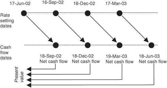
For the purposes of this exercise, you will receive fixed and pay floating on the very simple 1-year swap shown in Exhibit 6.1. Both fixed and floating payments are made quarterly (and so are netted) and fall on Eurodollar futures value dates. To simplify the upcoming analysis, fixed payments will be calculated using the fixed coupon and a fixed 90/360 day count fraction, while floating payments will be calculated using values of 3-month LIBOR together with an Actual/360 money market convention. And, although the fixed coupon on the swap does not depend on the swap’s notional principal amount, we will work with a $100 million notional amount for the purpose of calculating hypothetical cash flows.
EXHIBIT 6.1
1-Year Fixed/Floating Interest Rate Swap with Quarterly Payments
Everything you need to price and hedge this swap is provided by the Eurodollar futures market. First, the futures prices tell you the rates that you can lock in. Second, Eurodollar futures are the tools you, as a swap dealer, need to hedge any interest rate risk involved in taking one side or the other of the swap. As a dealer, you can agree to pay fixed and receive floating and offset your risk by buying Eurodollar futures. Or you can agree to receive fixed and pay floating and hedge your risk by selling Eurodollar futures. In either case, all you need to know is the fixed rate at which you can do the trade and break even.
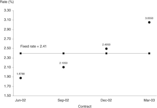
Consider the market data for June 17, 2002, that are shown in Exhibit 6.2. To price a 1-year swap, we will use the first four Eurodollar futures rates, which are plotted in Exhibit 6.3. The Jun ′02 contract price implied a 3-month rate of 1.8788%, which was also the spot value of 3-month LIBOR on that day. The Sep ′02 contract implied a rate of 2.105%, the Dec ′02 contract a rate of 2.495%, and the Mar ′03 contract a rate of 3.055%. Given these rates, which can be locked in using their respective contracts, the problem of pricing the swap is to find a fixed rate that is somewhere in the middle of the pack.
EXHIBIT 6.2
Eurodollar Futures Prices, Terminal Wealths, and Zero-Coupon Bond Prices
June 17, 2002
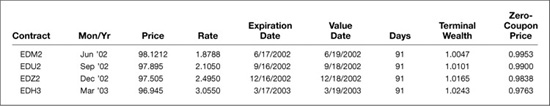
EXHIBIT 6.3
Eurodollar Futures Rates vs. Swap Fixed Rate
June 17, 2002
On balance, if you use the right fixed rate for the swap, you should find that any positive net cash flows will just offset any negative net cash flows. More to the point, the present values of cash flows on the swap should net to zero. In this example, this condition will be met if you find the fixed coupon, C, for which: where the Z’s represent the prices of Eurodollar zero-coupon bonds that mature on the four respective cash flow dates. These are available from Exhibit 6.2. Note that you use the price of a 3-month zero that matures on September 18 to value the first cash flow, the price of a 6-month zero that matures on December 18 to value the second cash flow, and so forth. If you plug the four zero prices into the equation, you can solve for C = 2.40670876% (see Exhibit 6.4).
EXHIBIT 6.4
Net Cash Flows and Present Values for a 1-Year Receive Fixed/Pay Floating Interest Rate Swap
Fixed Rate = 2.40670876%
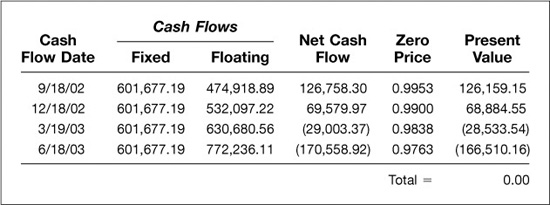
Exhibits 6.3 and 6.4 provide the comfort you need to know that this solution is correct. First, you can see from the chart in Exhibit 6.3 that the rate looks reasonable. It is higher than the first two of the Eurodollar rates and lower than the last two. Second, as shown in Exhibit 6.4, if we use the fixed rate to calculate the fixed cash flows on a swap with a notional value of $100 million and use the four futures rates to calculate the so-called floating payments, we find that the present values of the net cash flows sum to 0.00.
In practice, you may find that the rate at which you do a swap is higher or lower than what you have solved for here. For one thing, you are unlikely ever to encounter this much precision. For another, in real market situations, you and your counterparty may well be using slightly different market data. For yet another, you will encounter the effects of bid/asked spreads and uncertainties about the costs of hedging a swap position. For all of these reasons and more, your objective in doing a swap is to obtain terms that are favorable to you. If at all possible, in other words, you would like the swap to be struck at a rate that produces a positive net present value for you.
HEDGING A SWAP USING THE CASH FLOW METHOD
To hedge a swap using the cash flow method, the best way to start is to write out the net present value (NPV) of the swap in terms of cash flows and zero-coupon bond prices. Equation 6.1 shows that our 1-year receive fixed/pay floating swap has four cash flows and four zero prices. Armed with this expression, we can proceed to determine just how much the net present value of the swap changes as we vary each of the four futures rates. This, in turn, will allow us to calculate the hedge ratio for each of our futures contracts.
EQUATION 6.1
Find the 1-Year Swap Net Present Value Using the Cash Flow Method
NPV (Swap) = CF1Z1 + CF2 Z2 + CF3 Z3 + CF4Z4
where
CFi is the net cash flow for time i
Zi is the zero bond price associated with time i
What we will find is that a change in each of the rates will have two effects. The first, and primary, effect is the outright cash flow effect. If we are receiving fixed and paying floating, any increase in a floating rate before its rate setting date will cost us money. Thus, we are exposed to increases in the Sep ′02, Dec ′02, and Mar ′03 futures rates. We are not exposed to an increase in the Jun ′02 futures rate since June 17, our trade date, marks the Jun ′02 futures expiration and the rate setting date for our first cash flow.
The second, and secondary, effect is a sequence of present value effects. An increase in each of the rates will decrease the price of each zero-coupon bond that incorporates the rate. Note that even though the Jun ′02 contract expires as of the swap trade date, we are still exposed to changes in spot LIBOR. As a result, an increase in spot LIBOR will decrease the prices of all four zero-coupon bond prices, while an increase in the Mar ′03 rate will decrease only the price of the zero-coupon bond that matures on June 18, 2003.
The next step is to write out the partial derivatives (σ) to see how the swap’s net present value is affected by a change in each futures rate. The results of this exercise are shown in Equation 6.2.
EQUATION 6.2
Find the Change in the 1-Year Swap NPV Given a Change in Futures
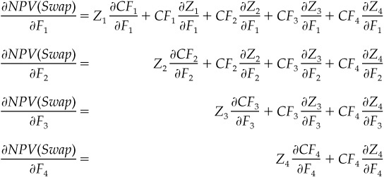
where
CFi is the net cash flow for time i
Zi is the zero bond price associated with time i
Fi is the futures rate for time i
Primary Effects
The first term in each of the four partial derivative equations represents the present value of the change in the floating cash flow given a change in the futures rate. The effect of a change in the rate on its associated cash flow is represented by σCFi/σFi, and the zero-coupon bond price we use to calculate the present value of the change is Zi.
The schematic provided in Exhibit 6.5 illustrates these cash flow effects. Note, first, that when the deal is done, the first cash flow is set so that changes in spot LIBOR will have no effect on the cash flow that falls in September 2002. The values of the next three cash flows are still variable, however. And, given the assumptions we have used so far in this example, a 1-basis-point increase in any of these three rates will produce a loss of $2,527.78 [= $100,000,000 × 0.0001 × (91/360)] in its associated cash flow.
EXHIBIT 6.5
Hedging the Swap’s Cash Flows June 17, 2002
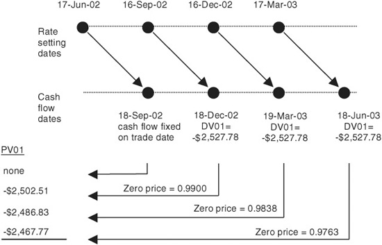
The time line presented in Exhibit 6.5 is very important for keeping the present values straight. For example, a change in the Sep ′02 rate affects the swap’s net cash flow on December 18, 2002, so we must use the price of a zero that matures on December 18 to determine the present value of the effect. A change in the Dec ′02 rate will, in turn, affect the March 19, 2003 cash flow, so we need a March 19 zero to value that change. And finally, a change in the Mar ′03 rate will affect the June 18, 2003 cash flow, so we need a June 18 zero to calculate the present value of that change.
We have, then, three variable cash flows, and, as shown in Exhibit 6.5, the present values of these effects depend on when they fall. The nominal or dollar value of a basis point (a.k.a. DV01) for each of the variable cash flows is a loss of $2,527.78, but the present value of a basis point (a.k.a. PV01) for each cash flow decreases with the length of the discounting horizon. The present value of the effect of a change in the Sep ′02 rate, for example, is a loss of $2,502.51 [= $2,527.78 × 0.9900], while the present values of changes in the Dec ′02 and Mar ′03 rates are losses of $2,486.83 [= $2,527.78 × 0.9838] and $2,467.77 [= $2,527.78 × 0.9763] respectively.
Secondary Effects
To complete the hedge, the next step is to determine the sizes and signs of the present value effects. In Equation 6.2, the secondary effects of a change in each futures rate on the zero-coupon bond prices are represented by σZi/σFi. A change in F1, for example, affects the zero prices associated with each of the four cash flows.
For someone who is receiving fixed when the yield curve is upward sloping, the early cash flows will tend to be positive so that any decrease in the zero price used to calculate its present value will be a loss. On the other hand, the later cash flows will tend to be negative so that any decrease in present values will be a gain. The results of these calculations are shown in Exhibit 6.6.
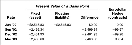
EXHIBIT 6.6
Swap Hedge Based on the Cash Flow Method
Effect of a 1-Basis-Point Increase in Each Futures Rate
June 17, 2002
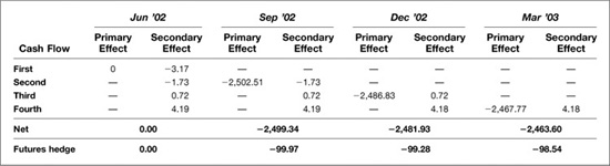
Because we are working with the swap’s net cash flows, these secondary present value effects are very small relative to the primary cash flow effects. A change in the Jun ′02 rate (spot or stub LIBOR) on balance has no effect at all. The losses on the first two positive cash flows are exactly offset by the gains on the last two negative cash flows. A change in the Sep ′02 rate, on the other hand, tends to offset very slightly the overriding cash flow effect. Taken together, these effects add to a gain of $3.18, which reduces the effect of a change in that rate on the swap’s net present value from $2,502.51 to $2,499.34.
Calculating Hedge Ratios
As usual, once you have done all the hard work of finding the present values of the effects of changes in the relevant futures rates, all that remains is to divide the results by $25, as shown in Equation 6.3. The results of these calculations are shown in the bottom row of Exhibit 6.6.
EQUATION 6.3
Find the Eurodollar Futures Hedge Ratios for the Swap
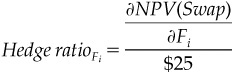
where
Fi represents the ith futures contract.
Hedge Ratios Are Dynamic
Eurodollar hedge ratios are dynamic, of course, and vary with changes in the level of interest rates and with the passing of time. (The effects of interest rates and time show up in the zero price, which is used to calculate the PV01.) As a result, your hedge ratios will tend to rise if rates fall because the prices of the zeros you use will tend to rise. Also, your hedge ratios will tend to increase with the passing of time because the present values of the variable cash flows will tend to rise.
PRICING A SWAP USING THE HYPOTHETICAL SECURITIES METHOD
At the outset of this chapter, we noted that the purpose of a swap is to mimic the cash flows on transactions that could just as well be carried out in the cash market. In this case, instead of receiving fixed and paying floating on a $100 million notional swap, you could have borrowed $100 million at 3-month LIBOR on June 17, 2002, and used the proceeds to buy a $100 million fixed rate note that would pay its fixed coupon in quarterly installments. In such an arrangement, the 3-month borrowing would have to be rolled over as each leg matures and refinanced at whatever 3-month LIBOR happens to be at the time. At the end of one year, the fixed rate note would also pay back its original principal of $100 million, which you would use to pay off the principal amount of the fourth leg of your short-term financing.
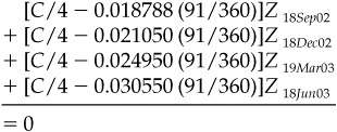
If you approach the problem of pricing the swap this way (and this is far and away the most popular and reliable way to price a swap), all you need to do is find the fixed coupon, C, at which the price of the hypothetical note would equal par. In this particular case, this would be accomplished if:
![]()
which can be rearranged as
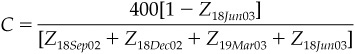
which also produces a solution of 2.40670876. Thus, the opening cash market trades that would begin to replicate the cash flows on the fixed/floating swap would be to borrow $100 million on June 17 at a spot LIBOR rate of 1.8788 and invest the entire $100 million in a 1-year note with a fixed coupon of 2.40670876. This way, the net initial cash flow would be zero (as it is with the swap) because the principal amounts offset each other perfectly. Thereafter, the net cash flows would be the difference between what you receive on the fixed rate note and what you pay on your floating rate financing. At final maturity, the principal amounts would offset again.
HEDGING A SWAP USING THE HYPOTHETICAL SECURITIES METHOD
Now we approach the problem of hedging the swap as if it were two hypothetical securities—a fixed rate asset financed with a floating rate liability. From the standpoint of someone with the position, the risk is not in the cash flows but in the values of the two securities. Of the two, the less risky is the floating rate liability, while the more risky is the fixed rate asset.
Floating Rate Liability
Consider the risks on June 17 once the two securities have been transacted. In the first place, you have a 3-month liability whose terminal value on September 18 will be
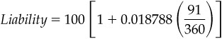
a value which is known today. At the instant the terms of the initial 3-month borrowing have been set, its present value can be represented as
where
Z18Sep02 represents the variable value of a zero-coupon bond that
matures on September 18 and whose price is
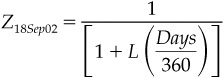
where
L represents the current (and variable) spot rate
Days is the total number of days from now until
September 18
In the middle of July, for example, L would represent a 2-month rate.
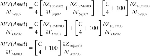
Fixed Rate Asset
The fixed rate asset represents four separate cash flows. The first three are straight coupon payments, each of which is worth C/4. The last is a combination of the final coupon payment and the bond’s principal. The present value of this asset can be expressed as
![]()
which is the same expression we used to price the swap in the first place.
When the swap is viewed this way, all of the relevant cash flows are fixed and only the spot and futures rates can vary. Finding the correct hedge ratios is then simply a matter of determining the effect of a change in each of the component rates on the net present value of the swap.
Find the Hedge Ratios
Consider first the effect of varying the value of spot LIBOR, which may be referred to as the “stub” LIBOR rate. The change in the present value of the liability would be:
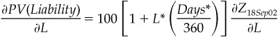
where
L* equals 0.018788 (fixed on trade date)
Days* equals 91 (fixed on trade date)
L represents the variable value of spot LIBOR
σ, borrowing from the calculus convention, represents a small change in whatever value follows it
Z is the zero-coupon bond price
The change in the present value of the asset would be
![]()
where
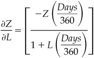
in which Days represents the actual number of days in the period covered by spot LIBOR. Taken together, the change in the net present value of the swap could be written as
![]()
Once you have dealt with your exposure to changes in spot LIBOR, the rest of the hedging problem looks fairly easy. Changes in the Sep ′02, Dec ′02, and Mar ′03 futures rates have no effect on the value of your short-term liability because they have no effect on the zero price used to value your liability. All that remains are effects on the value of your asset, which can be written as
where the Sep02, Dec02, and Mar03 subscripts correspond to the futures contract month and year.
The results of calculating these expressions are shown in Exhibit 6.7.
EXHIBIT 6.7
Swap Hedge Based on the Hypothetical Securities Method
Effect of a 1-Basis-Point Increase in Each Futures Rate
June 17, 2002
Writing out the interest rate effects this way helps to highlight the fact that coupon-bearing notes are more sensitive to changes in nearby forward rates than they are to changes in more distant forward rates. A change in the Sep ′02 rate, for example, affects the present value of three cash flows, while a change in the Dec ′02 rate affects the present value of two cash flows, and a change in the Mar ′03 rate affects the value of only one. As a result, when we solve for the hedge ratios, we find that we need fewer Dec ′02 contracts than Sep ′02 contracts, and we need still fewer Mar ′03 contracts.
Note, too, that the results of calculating the hedge ratios this way are exactly the same as those we derived using the variable cash flow approach. This is not an accident. Rather, it is because we took special care to express both hedging problems correctly and to keep track of all cash flow and present value effects in both problems.
This bears out a point made in the chapter on hedging with Eurodollar futures. That is, you can think of hedging as converting variable cash flows to fixed cash flows. Or you can think of hedging as converting variable present values to fixed present values. Either way, the two problems are really nothing more than two sides of the same coin and you should expect the answers to be the same.
PRICING AND HEDGING OFF-THE-MARKET SWAPS
So far in our analysis, we have dealt with swaps that are said to be on the market. These are swaps whose terms have been set at market and whose net present values are close to zero. Once the terms of a swap have been set, however, its value will rise or fall as the level of rates changes. And occasionally the fixed rate on a swap might be set above or below the current market level. In such cases, the net present value of the swap is not zero and the swap is said to be off the market.
Exhibit 6.8 shows how fixed coupons that are above or below the current market can affect the hedge for a swap. Consider, for example, a coupon of 0.4067 percent (0.004067), which is 2 percentage points below the market on June 17. If you are the counterparty who receives fixed, the swap is now a net liability; the swap’s present value is negative. In such a case, an increase in any of the four spot or futures rates that affect the present value of cash flows on the swap will reduce the present value of this liability, which would be a gain to you. You can see this in the upper panel of the exhibit, where an increase in spot LIBOR, for example, increases the net present value of the swap by $49.63. Similarly, you can see that the losses produced by increases in the Sep ′02, Dec ′02, or Mar ′03 rates are, on balance, smaller by roughly the same amount. As a result, the hedge would include a long position of 1.99 Eurodollar futures equivalent to hedge exposure to spot LIBOR and smaller short positions to hedge exposure to changes in each of the three futures rates. Overall, the total hedge would be net short approximately five fewer futures contracts.
EXHIBIT 6.8
Hedge for Below-the-Market Swap (0.4067%)
Effect of a 1-Basis-Point Increase in Each Futures Rate
June 17, 2002
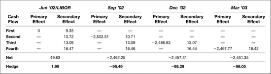
EXHIBIT 6.8
Hedge for Above-the-Market Swap (4.4067%)
Effect of a 1-Basis-Point Increase in Each Futures Rate
June 17, 2002
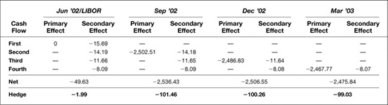
Similarly, if you were to receive a fixed coupon of 4.4067 percent, which is 2 percentage points above the market, the swap would represent a net asset. Increases in any of the four rates would decrease the net present value of your position, and as a result, your exposure to changes in rates would be increased. You would now need to short the equivalent of 1.99 futures to hedge your exposure to a change in spot LIBOR, and you would need larger short positions to hedge your exposure to each of the futures rates.
CONVEXITY DIFFERENCES BETWEEN FORWARD AND FUTURES RATES
We have seen several times throughout this chapter and in earlier chapters that Eurodollar hedge ratios tend to rise as interest rates fall and fall as interest rates rise. This tendency stems from the fact that the present values of cash flows rise when rates fall and fall when rates rise. For students of fixed income markets, this tendency is known as “positive convexity,” which describes the curvature in the relationship between the price of a non-callable bond and its yield as shown in Exhibit 6.9.
EXHIBIT 6.9
Convexity Characteristics of a Non-Callable Bond
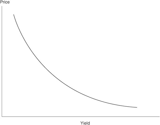
In contrast, Eurodollar futures have no convexity. The present value of a basis point is a fixed $25.00, which is entirely independent of the level of interest rates or the time to expiration of the Eurodollar futures contract.
The difference in convexity between non-callable fixed income instruments and Eurodollar futures is the source of dynamic hedge income for anyone who is long a non-callable bond or receiving fixed on a non-callable swap and who hedges the position by selling Eurodollar futures. For someone in the position, a decrease in rates increases the hedge ratio, which requires the hedger to sell more Eurodollar futures (and at a higher price). An increase in rates, on the other hand, decreases the hedge ratio, which requires the hedger to buy back Eurodollar futures (and at a lower price). Over time, as rates rise and fall at random, the hedger will pursue a dynamic hedging rule that involves selling futures as prices rise and buying futures as prices fall. The result is a trailing stream of hedging income that can be worth quite a lot if the process is allowed to run long enough.
The upshot of this difference between the positive convexity of non-callable fixed income instruments and the zero convexity one finds in Eurodollar futures is that futures rates must be higher than forward rates to compensate. That is, anyone who shorts Eurodollar futures must do so at a higher rate, and hence at a lower price, than the forward rate that determines the value of what one is hedging. Just how much this feature of Eurodollar futures is worth is detailed in chapters 7, 8, and 9, “The Convexity Bias in Eurodollar Futures,” “Convexity Bias Report Card,” and “New Convexity Bias Series,” which show how the value of the bias is tied to interest rate volatility and time to futures expiration.
For the purposes of this chapter, however, it is enough to know that if we are using Eurodollar futures rates to price swaps, we must first adjust them downward to net out the value of the bias. Exhibit 6.10, which is excerpted with permission from Carr Futures “Daily Zero to Ten” report, provides examples of how large the adjustments would have been on June 17, 2002. Contract by contract estimates of the value of the bias are shown in the column labeled “Bias.”
EXHIBIT 6.10
Estimating the Convexity Bias between Futures and Forward Rates June 17, 2002 Data as of 3:00 p.m. NY Close
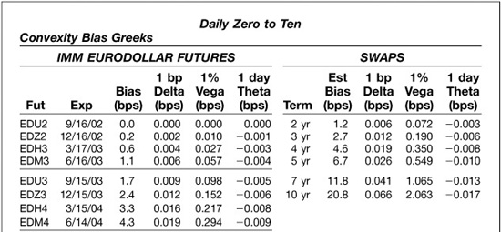
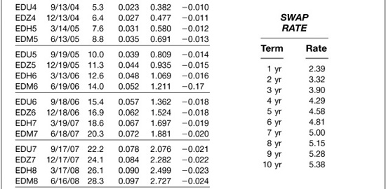
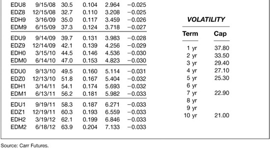
In this exhibit, the Jun ′02 contract has just expired, so the bias estimates begin with the Sep ′02 contract and end with the Jun ′12 contract. An examination of the convexity bias column shows the adjustment is very small for nearby contracts but increases exponentially as the time to a contract’s expiration increases. Thus, the adjustment for the Sep ′02 (EDU2) contract would be zero, while the adjustment for the Mar ′07 (EDH7) contract would be 18.6 basis points and the adjustment for the Jun ′12 (EDM2) contract would be 63.9 basis points.
The report also provides information about how sensitive the bias estimates are to changes in the level of interest rates (delta), the relative volatility of interest rates (vega), and the passing of time (theta). These sensitivity estimates are shown both for individual contracts and for swaps at key maturities. The report also includes the assumptions about interest rate volatility that have been used to calculate the bias estimates.
When pricing swaps, the results can be substantial. Exhibit 6.11 compares the results of calculating swap rates using both raw unadjusted futures rates and convexity-adjusted futures rates. And both are compared with market swap rates. For example, the 5-year swap rate (see swap maturity of Jun ′07) calculated from raw futures rates would have been 4.675%, while the rate calculated from the convexity-adjusted rates would have been 4.608%. The difference was 6.7 basis points. The market swap rate was 4.58%, which is much closer to the convexity adjusted rate than to the unadjusted rate.
EXHIBIT 6.11
Eurodollar Futures and Swap Convexity Bias
June 17, 2002
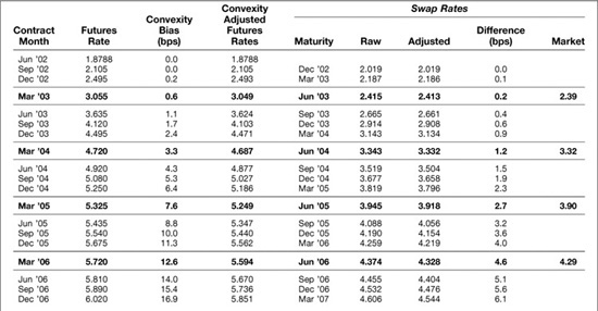
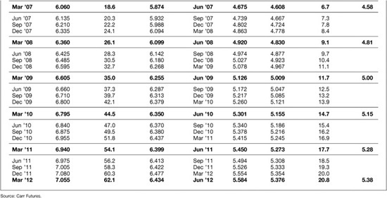
The difference is, of course, even more pronounced for a 10-year swap (see swap maturity of Jun ′12). The rate calculated from raw futures rates was 5.584%, while the rate calculated from convexity-adjusted futures rates was 5.376%. The difference was 20.8 basis points. The market rate was 5.38%, which was almost exactly the same as our convexity-adjusted rate.
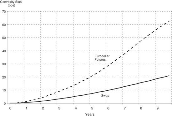
The value of the convexity bias is charted in Exhibit 6.12, which shows the value of the bias both by contract and for swaps of maturities ranging from 1 to 10 years.
EXHIBIT 6.12
Convexity Bias by Futures Contract and Swap Maturity
June 17, 2002
COMPARING THREE YIELD CURVES: FORWARD, ZERO COUPON, AND PAR COUPON
We now have all we need to conclude this chapter by comparing the three workhorse yield curves that one commonly finds in the fixed-income world—forward, zero coupon, and par coupon. Exhibits 6.13 and 6.14 show what these curves looked like on June 17 if derived from the Eurodollar futures market. The convexity-adjusted futures rates provide the futures market’s best guess about the values of the forward rates for each of the 40 3-month periods spanned by the 10 years in the table.
EXHIBIT 6.13
Three Yield Curves: Futures, Zero Coupon and Par Coupon
June 17, 2002
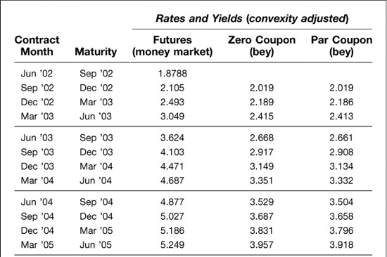

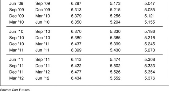
EXHIBIT 6.14
Three Yield Curves: Futures, Zero Coupon, and Par Coupon
June 17, 2002
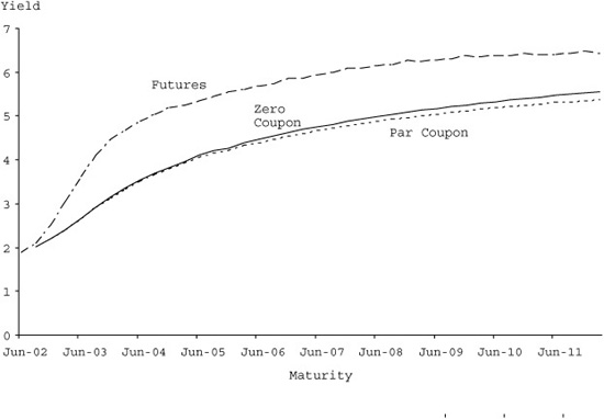
Next to the convexity-adjusted futures rates are the zero-coupon and par coupon yields that we have calculated from the convexity-adjusted futures rates. As one expects, with an upward-sloping yield curve, the zero-coupon yields are lower than the forward rates for each maturity, while the par coupon yields are lower than both. This is simply because the zero-coupon rates reflect a blend or average of the forward rates that go into the calculation of the term rate. In turn, a coupon rate is a weighted average of the zero-coupon yields that go into valuing each of the cash flows on a coupon-bearing bond.
The Difference between Money Market Rates and Bond Yields
The convexity-adjusted futures rates in Exhibit 6.13 are shown as quarterly money market rates, while the zero-coupon and par coupon yields are shown as semiannual bond equivalent yields (bey). We could have converted the money market rates to bond equivalent yields, or the bond equivalent yields to money market rates. We did not, however, mainly to make an important point.
Because yields are quoted in many different ways, a basis point in one market can be worth more or less than a basis point in another market. If we simplify the relationship between quarterly money market rates and semiannual bond yields as
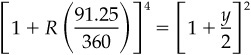
where R is the money market rate and y is the bond equivalent yield, we find that
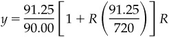
which says that the semiannual bond equivalent yield, y, will tend to be higher than the quarterly money market rate, R. By the same token, changes in bond equivalent yields will be larger than changes in money market rates. Or, what is the same thing, the value of a basis point is smaller if the reference rate is a bond yield than when the reference rate is a quarterly money market rate.
What this suggests, of course, is that you should avoid the mistake of calculating the value of a basis point using bond equivalent yields and converting the results into Eurodollar hedge ratios by dividing them by $25. The resulting hedge ratios will be too small. To avoid this mistake, it is better to follow the hedging procedures outlined in these chapters and reckon all values of a basis point in terms of quarterly money market basis points.