CHAPTER 13
Hedging and Trading with Eurodollar Stacks, Packs, and Bundles
SYNOPSIS
Eurodollar futures are the financial building blocks of the dollar interest rate market. With 40 quarterly contract expirations, the Eurodollar futures contract complex is a financial engineer’s dream. One can create or offset exposure to forward interest rates in 3-month segments out to a horizon of 10 years.
In practice, though, the flexibility afforded by individual contract expirations comes at a cost that is not always warranted. In many cases, traders and hedgers find it better to put all their eggs in one basket and use a single contract month (a stack). Or they may prefer to buy or sell packages of Eurodollar futures that the CME calls packs or bundles. A pack represents a sequence of 4 consecutive expiration dates that can be bought or sold simultaneously. A bundle is similar to a pack but spans 2 or more years’ worth of contract expirations.
Perhaps 15 percent or so of all trading in the first year’s expirations (that is, the white contracts) is done in the form of packs. Roughly half or more of all trading in expirations from 6 to 10 years (that is, the purple through copper years) is done in the form of packs or bundles. This suggests quite plausibly that the flexibility afforded by quarterly contract expirations is more important in the front months than in the more distant back months.
Three Objectives
We do three things in this note. The first is to provide a basic guide to the language and quote conventions of packs and bundles—the color coding of contracts and the way packs and bundles are bid and offered. The second is to take a look at the way pack and bundle hedges for Treasury notes perform. The third is to tackle the question of how a TED spread trade behaves when the trader introduces yield curve exposure by using a stack, pack, or bundle hedge in place of a hedge that is engineered to eliminate forward rate exposure.
How Good Are Stack, Pack, and Bundle Hedges?
Under normal circumstances, Eurodollar packs can do a very good job of capturing changes in the value of Treasury notes. The best pack hedges can provide correlations with daily changes in the prices of key Treasury notes that exceed 95 percent (see Exhibit 13.1). And, as we show later, you can get similar results with stacks and bundles. We also show how to scale a stack, pack, or bundle hedge to get a minimum variance hedge.
EXHIBIT 13.1
Treasury Note Correlations with ED Packs Daily Price Changes, June 1994 to June 1999

Curve-Augmented TED Spreads?
The decorrelation that accompanies a change in the slope or shape of the forward rate curve is a nuisance for hedgers but can be an opportunity for traders. For example, by hedging a Treasury note with a stack, pack, or bundle of Eurodollar futures, the trader can augment a standard TED spread with a yield curve trade. And because so many traders do just this, we take some time at the end of this note to tackle the problem of how one should measure the performance of a “curve TED” and to provide some evidence on how various curve spreads have behaved.
HEDGING AND TRADING WITH EURODOLLAR STACKS, PACKS, AND BUNDLES
Exhibit 13.2 shows five different Eurodollar hedges for the 5-1/2s of July 31, 2001, which was the on-the-run 2-year Treasury note on August 4, 1999. All five hedges have roughly the same number of Eurodollar contracts (net of whatever is needed to hedge the stub), but differ from one another in two key respects—ease of execution and yield curve exposure.
EXHIBIT 13.2
Eurodollar Hedges for a 2-Year Note
5-1/2s of 7/31/01 as of August 4, 1999
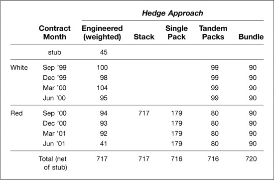
The engineered hedge is the most difficult to execute but is the combination of Eurodollar futures that is designed to capture as completely as possible the forward rate exposure in the 2-year note. A trader who buys $100 million of the note and sells this combination of Eurodollar futures will be long the term TED spread as conventionally defined. This position will profit from increases in the credit spread between the LIBOR and Treasury markets and will be almost completely unaffected by changes in the slope or curvature of the forward rate curve.
The stack, pack, and bundle hedges, in contrast, provide ease and economy of execution. Instead of the eight separate transactions required to put on the weighted hedge, the stack hedge requires only one transaction (the sale of 717 “red Seps”) as does the bundle hedge (the sale of 90 “2-year bundles”). The hedge can be done with the sale of 179 of a single pack such as “red Sep.” Or one could hedge with tandem packs with only two transactions (i.e., the sale of 99 “white packs” and the sale of 80 “red packs”). The drawback of these simpler hedges is a reduction in the quality of the hedge. Put differently, these simpler hedges inject curve exposure into the position, which will be an advantage to some hedgers and traders and a drawback to others.
BASICS: DATES, NAMES, PACKS, BUNDLES, AND QUOTES
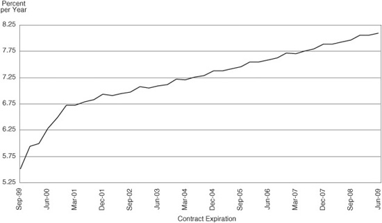
On any given day, the Chicago Mercantile Exchange lists 40 Eurodollar futures contract expirations in the March/June/September/December quarterly cycle. As Exhibit 13.3 shows, these 40 quarterly contracts, each of which is tied to its own value of 3-month LIBOR, span 10 years of the forward rate curve.
EXHIBIT 13.3
Eurodollar Futures Contract Rates Closing Levels, August 4, 1999
Contract Colors
Keeping track of 40 contracts in terms of expiration year and month is potentially very cumbersome. To simplify matters, at least for people who trade these contracts for a living, the CME defines expiration years in terms of a color-coded grid, with 4 contract expirations per color. On any trading day the first 4 quarterly contracts (the lead contract and the next 3 contracts that expire thereafter) are collectively dubbed the white year, or the whites. The next 4 quarterly expirations beyond the whites are called the reds. The 4 quarterly expirations beyond the reds are called the greens, and so on. As we move out to more distant expirations, the coding system vaguely resembles a 1965-vintage color TV. Exhibit 13.4 illustrates the complete color-coded grid, using contract expirations available on August 4, 1999. Note that the grid is dictated purely by the order in which futures contracts expire, not the calendar years in which they expire. Indeed, in only one quarter out of every four—the interval between mid-December and mid-March—will color-coded expiration years coincide with calendar years.
EXHIBIT 13.4
Contracts by Color August 4, 1999
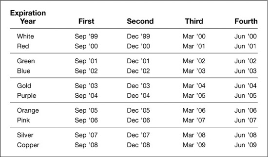
For generic purposes, we can reference a Eurodollar contract by color code of expiration year and contract position within expiration year, e.g., first red, or third green. That is the convention we will follow in the remainder of this note. Market transactors, however, typically name the contracts by color code of expiration year and month of expiration.
EXAMPLE
On August 4, 1999, we refer to the second blue contract as “blue Dec.” If we are also transacting in the first red contract, we refer to it as “red Sep.” The 4 contracts in the white year are generally referenced by only their month of expiration. Thus, if we are dealing in “March” on August 4, 1999, we are understood to be trading the third white contract.
Packs and Bundles
Frequently market practitioners wish to buy or sell entire sequences of Eurodollar futures contracts at once rather than transacting one contract expiration at a time. To accommodate such participants, the CME has introduced a variety of bulk transaction mechanisms, in the form of packs and bundles, that permit the simultaneous purchase or sale of equally weighted consecutive sequences of Eurodollar contracts.
Thus, a pack is a sequence of 4 futures contracts with consecutive expiration dates that can be bought or sold simultaneously. Market practitioners reference a pack by the member contract that expires soonest. On any given trading day, there are 37 packs available, ranging from first white out to first copper, and spanning all possible starting points in between.
EXAMPLE
On August 4, 1999, the red March pack comprises one each of the contracts expiring in March, June, September, and December of 2001 (i.e., red March, red June, green Sep, and green Dec). The gold Dec pack consists of one each of the contracts expiring in December 2003 and March, June, and September of 2004.
Any pack that is named simply by color code, without an expiration month, refers to the sequence of 4 contracts within the corresponding expiration year.
EXAMPLE
A broker who quotes a market in “the purple pack” is implicitly referring to the sequence of 4 contracts within the purple expiration year. On August 4, 1999, that comprises the contracts expiring between September 2004 and June 2005, making it identical in this case to the purple Sep pack.
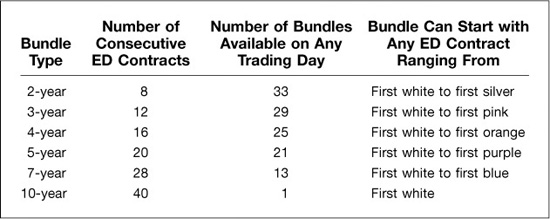
A bundle is mechanically similar to a pack, the chief difference being that the bundle spans 2 or more years’ worth of Eurodollar contract expirations, whereas the pack spans only 1 year’s worth. With a 5-year bundle, for example, a market participant can buy or sell one each of 20 consecutive Eurodollar futures contracts simultaneously (i.e., 5 years times 4 contract expirations per year). Market practitioners reference a bundle by (1) the member contract that expires first and (2) the length of the bundle in years. Exhibit 13.5 summarizes the types of bundles currently available.
EXHIBIT 13.5
The Menu of Eurodollar Bundles
EXAMPLE
On August 4, 1999, the red June 2-year bundle comprises 1 each of the 8 contracts that expire in June, September, and December of 2001, March through December of 2002, and March 2003. The green Sep 7-year bundle contains one each of the 28 contracts found in the 7 expiration years from green out to silver (i.e., all contracts from first green through fourth silver). The 10-year bundle—there can be only one—represents the sale or purchase of one each of the 40 quarterly Eurodollar contracts.
Any bundle that is named simply by year-length, without reference to any particular expiration month, is understood to refer to the lead (first white) bundle.
EXAMPLE
On August 4, 1999, a trader dealing in the “2-year bundle” is understood to have an interest in the bundle that comprises 1 each of the first 8 futures expirations, i.e., September 1999 through June 2001.
There are 122 possible bundles listed for trading on any given day.1 In practice, the more liquid of these are, with the exception of the 10-year, bundles within 5 years. At this writing, however, liquidity tends to be concentrated in just seven bundle configurations. Six of these are the lead (first white) versions of the basic bundle types listed in Exhibit 13.5. The seventh is the first purple 5-year bundle. Market practitioners call this bundle “L5” because it encompasses the last 5 years’ worth of contract expirations (first purple through fourth copper).
Note that market practitioners also are in the habit of referring to the pack that contains the first 4 contracts as the “1-year bundle,” not as the “white pack.” Early in the history of the pack/bundle trading facility, this distinction was meaningful. Today, however, it is purely an artifact of terminology. Thus, for convenience and consistency, we will call it the white pack throughout this note.
QUOTE PRACTICES 1: TICKS
The concept of tick is fundamental to understanding how markets are quoted in Eurodollar futures. One tick represents a move of 0.01 on a price base of 100.00. In interest rate (i.e., LIBOR) terms this corresponds to one basis point. A one tick move on a Eurodollar contract is always worth $25, regardless of the contract’s expiration date.
EXAMPLE
If a Eurodollar futures contract price moves from 93.20 to 93.25, it has rallied 5 ticks. The corresponding contract rate (in LIBOR terms) has declined 5 basis points, from 6.80 percent per year to 6.75 percent. If we own 100 of this contract, then we will collect a variation margin adjustment of $12,500 [= $25/tick × 5 ticks/contract × 100 contracts]. Conversely, if we have a short position in the same 100 contracts, then we must pay $12,500 in variation margin adjustment.
The value of a 1-tick move for a pack or a bundle is simply $25 times the number of contracts in the pack or bundle.
EXAMPLE
If we have a short position in 100 4-year bundles (any 4-year bundle) that has risen in price from 93.18 to 93.195, then we are liable for a variation margin payment of $60,000 [= $25/tick × 1.5 ticks/contract × 16 Eurodollar contracts/bundle × 100 bundles].
QUOTE PRACTICES 2: USE PRICE LEVEL FOR INDIVIDUAL CONTRACTS
Individual Eurodollar contracts are traded in terms of price, with the tick as the basic unit of measure.
EXAMPLE
On the afternoon of August 4, 1999, market players bid the Dec ′99 contract at a price of 94.06 and offer it at 94.07. Traders and brokers will quote this as a “six-seven” market. If the market tightens to 94.06 bid versus 94.065 offered, they will quote it as “six-six-and-a-half” or “six to the half.”
Though the tick is the basic unit of measure, it is not the smallest unit. On most days all Eurodollar contracts trade in half ticks. The sole exception is the lead contract, which is permitted to trade in quarter ticks during the 4-week interval immediately preceding its expiration. (To be more precise, the lead contract trades in quarter ticks during the interval starting with the Monday before the third Wednesday of the previous month, i.e., the expiration day of the previous month’s serial futures contract, and ending with the contract’s own expiration. Though this interval typically spans 4 weeks, the vagaries of the calendar sometimes stretch it to 5.)
QUOTE PRACTICES 3: USE PRICE CHANGES FOR PACKS AND BUNDLES
The daily settlement prices that are established at 2:00 p.m. Chicago time play a pivotal role in how packs and bundles are quoted, for two reasons. First, it is at this point in the trading day that actual price levels are set for all packs and bundles. The price of each pack or bundle is simply the arithmetic average of the prices of its member contracts.
EXAMPLE
On August 4, 1999, the CME records the following closing price levels:
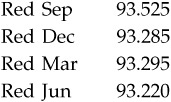
To determine the closing price level of the red pack, CME officials compute the arithmetic average of the closing prices on these 4 individual contracts, which is 93.33125.
Second, and more important, is that over the ensuing 24 hours the market price of any pack or bundle will be quoted in terms of tick change versus the previous day’s 2:00 p.m. Chicago time settlement level. (It is useful to recall here that the Eurodollar futures market trades more or less continuously—by open outcry during regular trading hours [7:20 a.m. to 2:00 p.m. Chicago time], and on GLOBEX nearly continuously [4:30 p.m. to 4:00 p.m. next day, Chicago time].)
As with Eurodollar futures contracts, packs and bundles trade in smaller increments than one tick. However, the finest permissible price move for any pack or bundle is a quarter tick versus the half tick minimum move that applies to individual contracts.
It is early on August 5, 1999, and mid-market prices for contracts in the red pack are as follows—
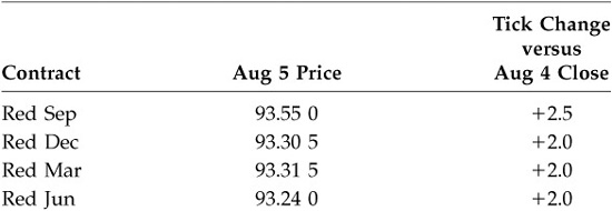
The average price change across these 4 contracts is a gain of +2.125 ticks. That is where market participants will be inclined to price the red pack. However, they will be unable to quote it as “up two and an eighth” because the pack is constrained to move in price increments of a quarter tick or more. Thus, they will have to quote it as “up two,” or as “up two and a quarter,” or as a bid/offer spread, e.g., “up two to the quarter.”
UNPACKING PACKS, UNBUNDLING BUNDLES
A pack or bundle exists only up to the point that it has been transacted. It does not show up as a package on the books of its buyer and seller. Rather, the Eurodollar contracts in the package are booked individually, at transaction prices that are consistent with the average price at which the pack or bundle changed hands. For this reason, anyone who employs these bulk transaction mechanisms should have a clear understanding of how their prices get translated into individual contract prices.
Once a buyer and a seller have agreed upon the price of a pack or a bundle, they must assign mutually acceptable prices to each of the contracts in the package. In principle, the transactors may set these component prices arbitrarily, subject to two restrictions.
The first and more obvious one is that the average price change among the contracts (versus their previous 2:00 p.m. CT closing levels) must equal the price change at which the pack or bundle has been priced.
Second, the price of at least one Eurodollar contract must lie within that contract’s trading range for the day (assuming that at least one of the Eurodollar contracts in the pack or bundle has established a trading range). This rule ensures that the prices of bulk transaction devices remain tethered to the price action of the underlying individual Eurodollar contracts.
EXAMPLE
Suppose we have sold the 2-year bundle (i.e., 1 each of the 8 contracts in the white and red expiration years) to a buyer at the price of +5 ticks. In principle, we can agree with the buyer to unbundle this average price change as +10 ticks on each of the 4 white contracts and zero price change for each of the 4 red contracts (assuming of course that such pricing fulfills the trading-range constraint mentioned above). Alternatively—again, in principle—we can agree with the buyer to exchange each of these 8 contracts at a price change of +5 ticks.
Rarely in practice do market participants spend time dickering over how to price the individual members of the packs or bundles that they have traded among each other. The objective in using these devices, after all, is to save time. Instead, they almost always rely on a computerized system furnished by the CME that automatically assigns individual prices to the contracts in any pack or bundle.
The algorithm employed by the CME’s pricing system is guided by the following principle: To the extent that adjustments are necessary to bring the average price of the pack’s or bundle’s components into conformity with the bundle’s own price, these price adjustments should begin with the most deferred contract in the bundle and should work forward to the nearest contract.
EXAMPLE
Suppose that a buyer and a seller who are transacting in the 3-year bundle have agreed upon a net price change of −2.75 ticks versus the previous day’s settlement level. The CME algorithm distributes this price change among the bundle’s 12 member contracts in two steps, dealing first with the integer portion of the −2.75 tick trade price (the “2”), and then with the fractional portion (the “0.75”). Specifically, the algorithm begins by assigning to each of the 12 contracts in the bundle a net price change of −2 ticks from the previous day’s close. Then it adjusts these price changes downward, proceeding one contract at a time—beginning with the bundle’s most deferred contract and working forward—until the average net price change for the bundle is the agreed-upon −2.75 ticks. Following this procedure results in the bundle’s nearest 3 contracts being booked at prices that are −2 ticks below their respective closing levels for the previous day, while the bundle’s 9 most deferred contracts are each booked at net price changes of −3 ticks. The average price change across the 12 contracts is (9 × −3 + 3 × −2)/12 = −2.75 bps, as desired.
Note that although futures contracts trade in half ticks, the CME price-distribution algorithm works only through whole-tick price adjustments.
The relentless efficiency of the Eurodollar futures market means that the price change quoted for a pack or a bundle will almost never deviate systematically from the actual average price change across the individual contracts within the pack or bundle. However, the two are apt to exhibit frequent short-lived deviations, ranging in size from as much as 1/4 contract tick to as little as 1/80 contract tick (on a 10-year bundle). These will arise as natural artifacts of the restrictions on minimum price increments—half ticks for individual Eurodollar contracts versus quarter ticks for packs and bundles.
EXAMPLE
Just before 2:00 p.m. Chicago close on August 5, 1999, we want to buy 1 each of the first 8 Eurodollar futures. Price changes among these contracts versus their August 4 closing levels range from +3 ticks on white Sep to +9-1/2 ticks on white Mar. Their average price move is +6-5/16 ticks. We can buy them individually, but we also consider buying them as a 2-year bundle. Since the bundle is constrained to trade in increments of 1/4 tick, it cannot be priced at +6-5/16 ticks. Rather it is apt to be quoted at either +6-1/4 ticks or +6-1/2 ticks. If we can buy the bundle at +6-1/4 ticks, then we enjoy an overall discount of −1/16 tick per contract by using the bundle instead of purchasing the 8 contracts individually. (By contrast, if the Eurodollar pit offers the 2-year bundle at +6-1/2 ticks, then it is not such a great deal. We would pay a premium of +3/16 tick per contract to buy our futures contracts in bundle form instead of individually.) Having bought the bundle at +6-1/4 ticks, suppose we apply the CME’s price distribution algorithm in unbundling it. If we do this, we will pay +6 ticks for the first 6 contracts (white Sep through red Dec) and +7 ticks for the last 2 (red Mar and red Jun).
For more on the basics of Eurodollar futures, packs, and bundles, see “CME Interest Rate Futures: The Basics,” from the Chicago Mercantile Exchange.
HEDGING WITH STACKS, PACKS, AND BUNDLES
The engineered hedge shown in Exhibit 13.2 is designed to eliminate as completely as possible any yield curve exposure in the hedged position. All the risk that remains stems from changes in the credit spread, which in this case would be the 2-year term TED spread.
Simple stack, pack, and bundle hedges will work less well than will engineered hedges. This is because rate changes across contract months are not perfectly correlated.
Also, the total number of contracts needed to produce the “best” stack, pack, or bundle hedge—that is, the hedge with the smallest variance—may well be more or less than the number required for the engineered hedge. For one thing, a hedger faced with imperfect correlations can improve things by underhedging. For another thing, rate changes tend to be larger for some contract months—for example, the red months—than for others. As a result, the hedger will want to scale the size of the hedge up or down to compensate for any regular differences in rate variability.
What Happens to the Correlations?
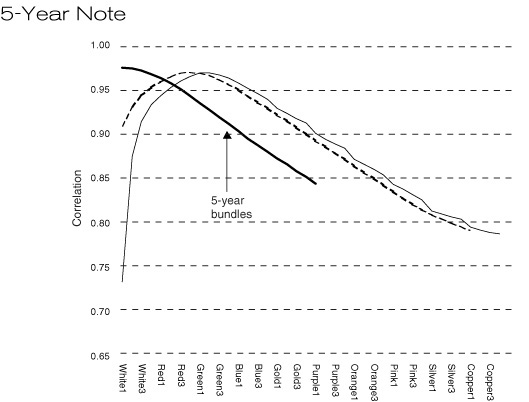
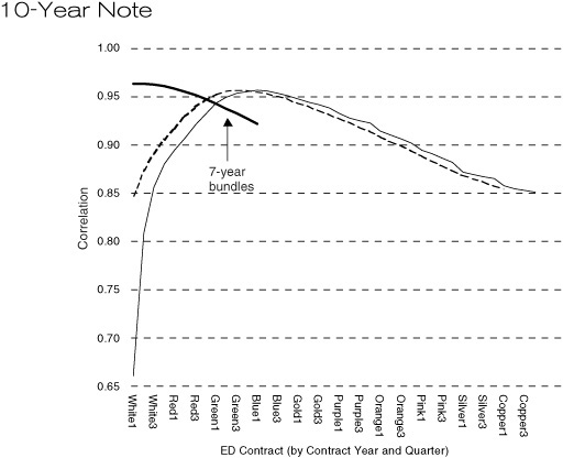
Exhibit 13.6 shows how changes in the values of various stack, pack, and bundle hedges correlate with changes in the values of on-the-run 2-year, 5-year, and 10-year Treasury notes. One can see easily which of these hedges provided the best protection and how much the correlations fall off if the hedger chooses something other than the best spot on the curve.
EXHIBIT 13.6
Best Pack and Bundle Hedges
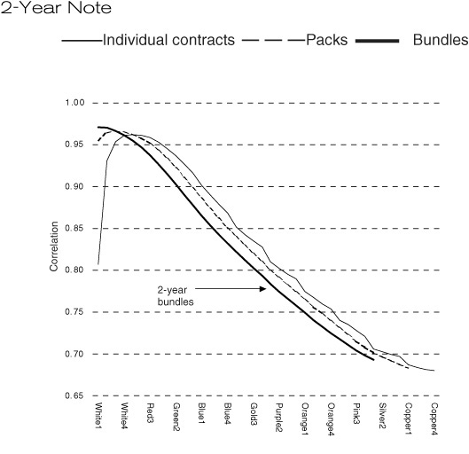
These rankings are based on correlations between day-to-day changes in (clean) prices of Treasury notes and day-to-day changes in the prices of Eurodollar futures contracts or packs or bundles. The “best” futures hedge for a given Treasury note is simply the ED package most highly correlated with it. (Specifically, the data we use to compute these correlations are daily changes—from futures close to futures close—in prices of ED futures and (clean) prices of Treasury notes over the 5-year interval from mid-June 1994 to mid-June 1999. Note that this span of history is sufficiently long to embrace a broad variety of market environments—bullish, bearish, stable, volatile. At the same time, it is reasonably homogeneous in terms of the Fed’s operating procedures and policy announcement protocols.)
Three things are apparent from Exhibit 13.6. First, the best of these stack, pack, and bundle hedges are really quite good, at least under normal circumstances. In all cases, the highest correlations are between 0.95 and 1.00. If one allows for the fact that even the engineered hedge would exhibit a correlation that is less than 1.00 because of residual credit spread or TED spread risk, the hedger does not lose much at all.
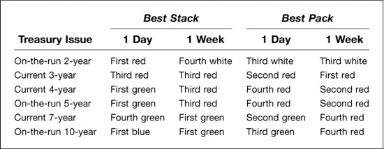
Second, the best stack, pack, or bundle hedge is found at different, and in some cases surprising, places on the Eurodollar curve. For example, although it is impossible to see in Exhibit 13.6, the best 2-year bundle hedge for the on-the-run Treasury began with the second white contract, not with the lead, or first, white contract. As shown in Exhibit 13.7, the best stack hedge for the 2-year note was the first red contract, and the best pack hedge was the third white pack.
EXHIBIT 13.7
Best Single Contract, Pack, and Bundle Hedges
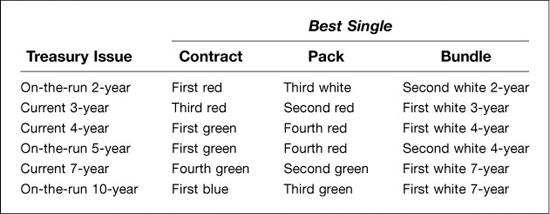
As one would expect, the best stack, pack, or bundle hedge for a 5-year or 10-year note is further out along the Eurodollar curve than is the best hedge for the 2-year note. As shown in Exhibit 13.7, the best stack hedges would be the first green and first blue contracts for these notes. The best pack hedges began with the fourth red and third green contracts.
Third, the term of the best bundle does not always correspond to the maturity of the note. For example, the best bundle hedge for the on-the-run 5-year note was not, as one might expect, a 5-year bundle. Rather, the second white 4-year bundle produced a slightly higher correlation than did any of the 5-year bundles.
Best Pack Proxies for Key Treasury Maturities
How well can Eurodollar packs capture the behavior of yields at key points along the Treasury curve? The high correlations of the best pack hedges shown in Exhibit 13.8 would suggest that packs can do a very good job of representing Treasurys.
EXHIBIT 13.8
Treasury Note Correlations with ED Packs Daily Price Changes, June 1994 to June 1999
A closer look tells us, though, that they would not do a very good job of discriminating. For example, the best pack hedge for the current 4-year note and the on-the-run 5-year note is the fourth red pack. Note, too, that the best pack hedge for the on-the-run 10-year note is the third green pack, which is only 3 contracts, or 9 months, farther out on the Eurodollar curve than the fourth red pack. Thus, using correlation alone to find the best proxy for a Treasury note would be no help at all in trading the 4-year/5-year Treasury spread, and would be comparatively little help in the trading the 5-year/10-year spread.
Horizon Matters
When using changes in rates or prices to estimate correlations, it makes sense to us to match the period over which one calculates changes with the hedging horizon. For example, if a typical position is held for a day, then daily changes seem best. If a position is held for a week, then weekly changes seem best.
As shown in Exhibit 13.9, the best stack or pack hedges depends somewhat on the hedging horizon. For example, the best 1-day pack hedge for the on-the-run 5-year Treasury was the fourth red pack. The best 1-week pack hedge was the second red. The differences shown in Exhibit 13.9 are not especially large, but the best hedges using weekly changes do tend to be closer in on the Eurodollar curve.
EXHIBIT 13.9
Hedge Horizon and Best Hedges
The Dangers of Decorrelation
Whoever said that the only thing that goes up in a crash is correlations was not thinking of stack, pack, and bundle hedges.
In recent years, short-run estimates of correlation between Treasury notes and Eurodollar futures have rarely strayed too far from their long-run benchmarks. Consider, for example, the relationship between the Treasury 5-year note and the 5-year Eurodollar bundle, as depicted in Exhibit 13.10. The jagged line represents a running correlation of daily changes estimated over 20-day periods. The solid straight line represents the full period correlation, which was 0.975. And, over most of the 5 years covered by Exhibit 13.10, the running 20-day correlation was higher than this.
EXHIBIT 13.10
Short-Term versus Long-Term Correlation between Price Changes in 5-Year Treasurys and First White 5-Year Bundle
Daily, June 14, 1994 to June 14, 1999
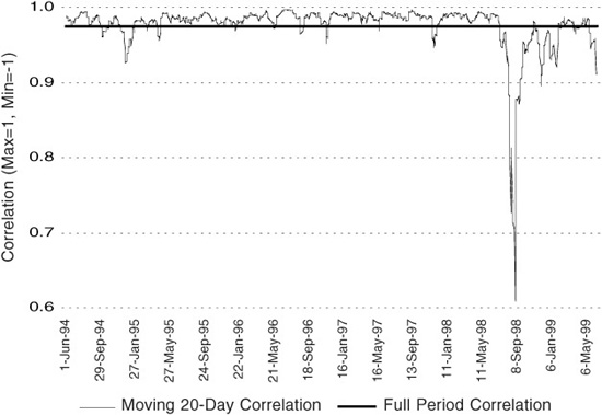
Exhibit 13.10 also shows what can happen to correlations if things go badly, as they did in the autumn of 1998 when credit markets were roiled by Russia’s financial meltdown and the failure of Long-Term Capital Management. The typically rock-steady relationship between the 5-year T-note and the 5-year ED bundle deteriorated abruptly, with the correlation between them plunging almost to 0.60 from values that were almost 1.00.
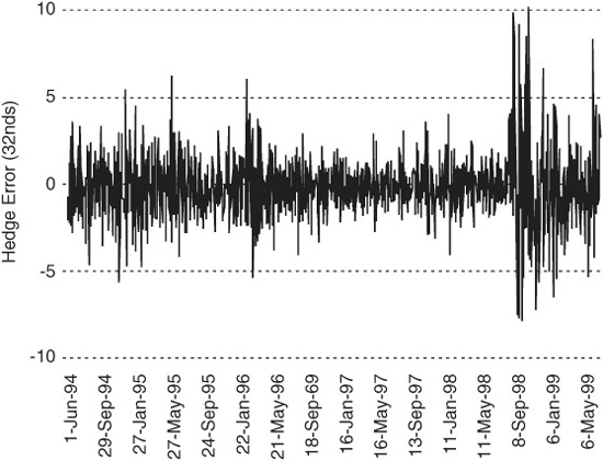
What this means in dollars and cents is shown in Exhibit 13.11, which depicts daily hedge errors for a hypothetical trader who is always long the on-the-run 5-year T-note and is short an appropriate number of 5-year Eurodollar bundles. Through the 4 years from mid-June 1994 to mid-June 1998, the hedge errors on this trade ran reliably close to zero, typically less than 2/32nds. The plunge in correlation in late summer and early fall of 1998 caused a correspondingly sharp jump in range and variability of hedge errors.
EXHIBIT 13.11
The Consequences of Decorrelation:
Errors from DV01-Hedging OTR 5-Year Treasury Note with First White 5-Year Bundle
Daily, June 14, 1994 to June 14, 1999
Scaling Your Hedges to Reduce Hedge Error
Once you decide to use a stack, pack, or bundle in lieu of an engineered hedge, you may want to consider scaling the hedge to compensate for two things—differences in rate variability and a loss of correlation. It is useful to think of a hedge ratio as the product of two things—the correlation between the two variables and the ratio of their respective standard deviations (i.e., beta). For example, if you want to hedge y with x, the hedge ratio that you would find by regressing y on x would be:
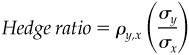
where ρy, x is the correlation between y and x, and σy and σx are the standard deviations of y and x respectively.
The handy thing about this way of expressing the hedge ratio is that two things are readily apparent. First, if the two variables are perfectly correlated, the hedge ratio is simply the ratio of the two standard deviations. Second, if the two variables are less than perfectly correlated, the hedge ratio will be smaller than the ratio of the standard deviations.
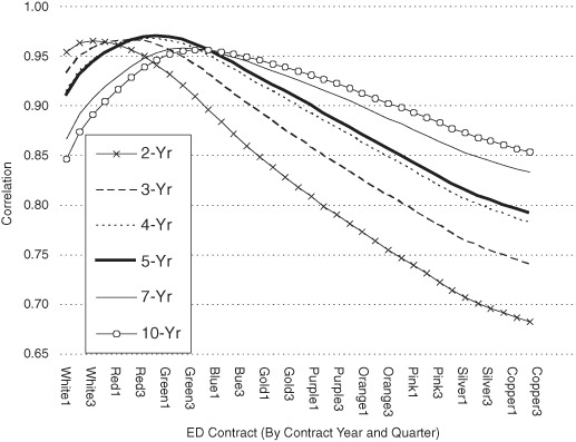
Both forces come into play when hedging with stacks, packs, and bundles. Consider the results shown in Exhibit 13.12. The curve represents the standard deviation of daily changes in individual Eurodollar contract rates. The two solid squares represent the standard deviation of daily changes in the yields of hypothetical 2-year and 5-year Eurodollar bonds.
EXHIBIT 13.12
Volatility of Daily Changes in ED Contract Rates and Term TED Yields
Standard Deviations, Mid-1994 to Mid-1999
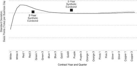
The shape of the curve illustrates three key features of Eurodollar rate volatility. First, the lead contract (i.e., the first white contract) is the least variable of all. The red contracts tend to be the most volatile of all. And once you get past the greens, all rates exhibit roughly the same variability.
The practical consequences for hedgers are clear. If you want to hedge a 2-year note with any red stack or red pack, you will need fewer contracts than are called for in the engineered hedge. Or if you want to hedge a 5-year note with a gold stack or pack, you will need more contracts than are called for in the engineered hedge.
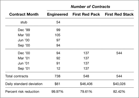
Taken together, imperfect correlations and differences in variability of rate changes across contract months encourage the scaling of hedges. For example, as shown in Exhibit 13.13, the engineered hedge for the on-the-run 2-year note would eliminate nearly all of the forward rate exposure in the note. (The percent risk reduction shown in Exhibit 13.13 applies only to rate risk, not to credit spread risk.) As shown, the engineered hedge would require 738 contracts. In contrast, the best red pack hedge would use only 548 contracts and at this size would reduce the forward rate risk in the position by 20 percent. More or less than this number of contracts would add risk to the hedge. By the same token, the hedger would require only 544 of the first red contract to get a minimum risk hedge.
EXHIBIT 13.13
Scaled Hedges for a 2-Year Treasury Note
5-5/8s of 9/30/01 as of October 27, 1999,
Daily Standard Deviation = $227,618
TRADING CURVE TEDs
Some people look at the curve mismatches implied by stack, pack, and bundle hedges for Treasurys and see opportunities instead of problems.
Up to this point, we have assumed that the practitioner wants to construct a hedge with whatever Eurodollar futures package (contract, pack, or bundle) is most highly correlated with his Treasury note. For a hedger interested in minimizing basis risk, this is the right approach. It may not, however, suit the purposes of a speculative trader for whom a certain amount of decorrelation between Treasurys and Eurodollar futures is necessary for profitable trading opportunities to exist.
The challenge then for the speculator—or for the hedger who wants to improve the odds—is to identify, for any given Treasury note, which curve TEDs are out of line and whether they are sufficiently out of line to offer the prospect of a profitable trade.
The best way to understand how a curve TED spread trade works is to break it down into its two components—a standard weighted TED spread trade and a Eurodollar curve spread trade.
Curve TED = Standard TED + Curve spread
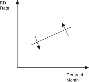
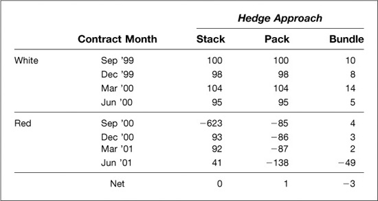
Consider, for example, the curve TED trade illustrated in Exhibit 13.14. In this case, the trader buys a 2-year Treasury note and sells 179 of the red pack. This trade can (and should) be thought of as the sum of two separate trades. First, as shown in the middle column, the trader is long the standard 2-year term TED spread, which is long the 2-year note and short a weighted strip of Eurodollar futures. Second, as shown in the right-hand column, the trader is long the white contracts and short the red contracts and is, as a result, long the slope of the 2-year Eurodollar curve. The standard 2-year term TED will profit from an increase in the pure credit spread between LIBOR and Treasury yields. The curve spread will profit if the 2-year segment of the Eurodollar futures rate curve steepens as shown in Exhibit 13.15. For this part of the trade to profit, “red” futures rates must rise relative to “white” futures rates.
EXHIBIT 13.14
Deconstructing a Curve TED Spread
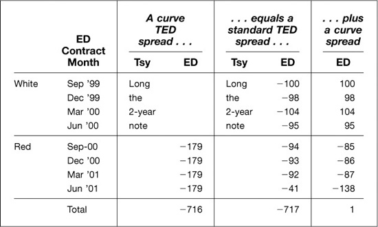
EXHIBIT 13.15
The Curve Trade Implied by a Red Pack Hedge for a 2-Year Treasury Note
Calculating the Hybrid Spread
Tracking the performance of a curve TED requires a consistent measure of the value of the hybrid spread. Perhaps the best and simplest way to do this is to begin with a measure of the standard TED spread. To this can be added the difference between the average rate at which the trader is short Eurodollar futures and the average rate at which the trader is long Eurodollar futures in the curve part of the trade. For this kind of addition to work correctly, the two spreads should be quoted in like terms. Since the curve spread is an average of quarterly money market rates, any measure of the TED spread that is measured in semiannual bond equivalent yield terms (for example, the implied yield and implied price TEDs that one finds on Bloomberg) should be converted to quarterly money market basis points. Or one could use the spread-adjusted TED (what we call the fixed basis point spread to Eurodollar rates), which is quoted in quarterly money market basis points by definition. Or, finally, one could convert the Eurodollar curve spread from quarterly money market basis points into semiannual bond equivalent basis points. In this note, we express everything in money market terms.
A correct reckoning of the curve spread requires only that the value of a basis point change in the value of the curve spread be the same as the value of a basis point change in the standard TED spread. In this example, the standard weighted hedge for the Treasury note has a total of 717 Eurodollar contracts so that the value of a basis point is $17,925 [= 717 contracts × $25 per contract per basis point]. Thus, for the purposes of calculating the curve spread, we should think of the curve trade in terms of the gross trades needed to add the curve trade.
As shown in Exhibit 13.16, the curve trade we are adding to the TED trade could be accomplished by buying the strip of Eurodollar futures shown under the “long” column and selling the strip of Eurodollar futures shown under the “short” column. (The actual trade would simply be the net of these two strips.) Given these contracts and the closing values of the Eurodollar contract rates for August 4, the average rate at which the trader is short is 6.669 percent, and the average rate at which the trader is long is 6.244 percent. The difference is 0.425%, or 42.5 basis points, which can be added to the value of the 2-year term TED spread, which was 71.4 basis points. Taken together, the value of the curve TED spread would be 113.9 basis points [= 71.4 + 42.5].
EXHIBIT 13.16
Calculating the Curve Spread
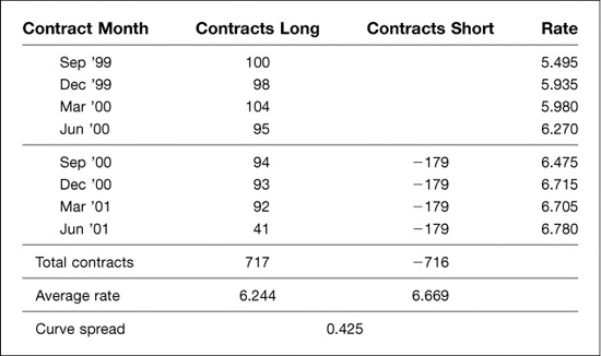
Similar adaptations of the standard TED spread can be done for other kinds of TED hedges. For example, if the trader decided to hedge the 2-year note with the first red stack, the curve exposure would be an odd sort of butterfly, as shown in Exhibit 13.17. To achieve this, the trader could be thought of as buying back the original Eurodollar strip and selling 717 of the first red contract (red Sep in this case). Thus, the trader would be short at a rate of 6.475 percent (the rate for the red Sep contract in Exhibit 13.16) and long at an average rate of 6.244 percent. The curve spread would then be 0.231 percent, or 23.1 basis points.
Looking for Opportunities
If the trader wants to augment a standard TED spread with a curve spread, the next challenge is to find the best opportunities. One perspective is provided by the change in a particular kind of curve spread through time. Exhibit 13.18, for example, shows how generic versions of the stack, pack, and bundle curve spreads described in Exhibit 13.17 behaved over the past 5 years. Not too surprisingly, the curve spread produced by substituting a 2-year bundle for the engineered hedge was very stable. Rarely, for that matter, was this curve spread more than 2 or 3 basis points.
EXHIBIT 13.18
Generic Eurodollar Curve Spreads
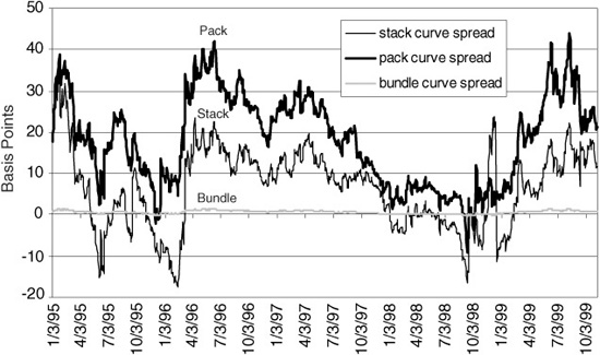
The stack and pack spreads, on the other hand, proved to be really quite volatile. In the stack curve spread, for example, you can see the curvature of the forward rate curve increase and decrease as the value of the spread rises and falls. And, in the pack curve spread, you can see the slope of the forward rate curve increase and decrease as the value of the spread rises and falls.
The effect of appending the pack curve spread to a conventional 2-year TED spread is illustrated in Exhibit 13.19. The lightest line tracks the value of the 2-year TED spread, and the darkest line tracks the value of the pack curve spread. The value of the augmented pack curve TED is traced out by the third line. In this history, the two components of the pack curve TED exhibit a considerable degree of independence. Over the period shown, the correlation of weekly changes in the values of the 2-year TED spread and the pack curve spread was 0.10.
EXHIBIT 13.19
Augmenting a 2-Year TED Spread
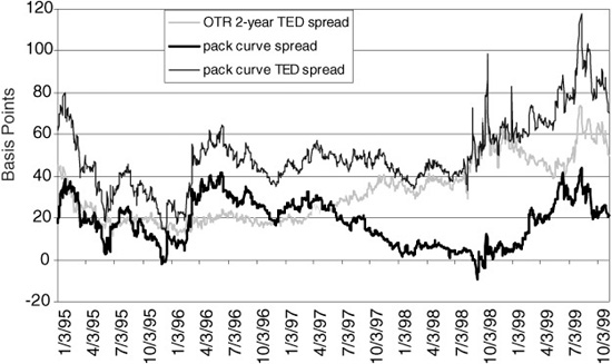
To the extent the two components of the pack curve TED spread are uncorrelated, the pack curve TED spread will have desirable risk/return characteristics. A curve TED spread represents a diversified portfolio of two separate spreads—namely the pack curve spread and the conventional TED spread. Thus, during those intervals when the pack curve spread and the conventional TED spread are uncorrelated with each other, the pack curve TED should exhibit less risk for any given expected return than will the conventional TED spread by itself.
Consider the recent experience with both parts of the spread trading at historically rich levels—that is, the 2-year TED spread above 60 basis points and the pack curve spread above 40 basis points. At these values, a trader could have sold either of the spreads by themselves. Combining them, though, by selling a Treasury note and buying red packs could have produced a trade with the same potential gain but with less risk.
In this case, the trade opportunity is presented by a steepening of the Eurodollar rate curve in the white and red years. In augmenting a TED trade, one has a much longer menu of curve trades from which to choose.