
CHAPTER 23
Trading with Serial and Mid-curve Eurodollar Options
SYNOPSIS
Serial and mid-curve Eurodollar options have been available at the Chicago Mercantile Exchange (CME) for a number of years. These options, which expire anywhere from 1 month to 2 years before their underlying futures contracts expire, open up whole new realms of trading opportunities, which, until recently, went largely unexploited owing to a lack of liquidity. Lately, however, trading volume and liquidity have picked up noticeably, as more and more traders have recognized that these options enable them to achieve exposures never before attainable with exchange-listed options. The main distinguishing feature of these options is that they provide high-gamma, high-theta vehicles for trading various segments of the futures or forward rate curve. This note explains some of the many uses for these products.
The array of options available for trading on March 25, 1998, is shown in Exhibit 23.1. Option expirations are displayed along the top with futures expirations along the side. The options are labeled using the names by which they are identified on the CME floor. March 25 closing bid and offered implied volatilities appear in parentheses below each option’s name.
EXHIBIT 23.1
Quarterly, Serial, and Mid-curve Eurodollar Options
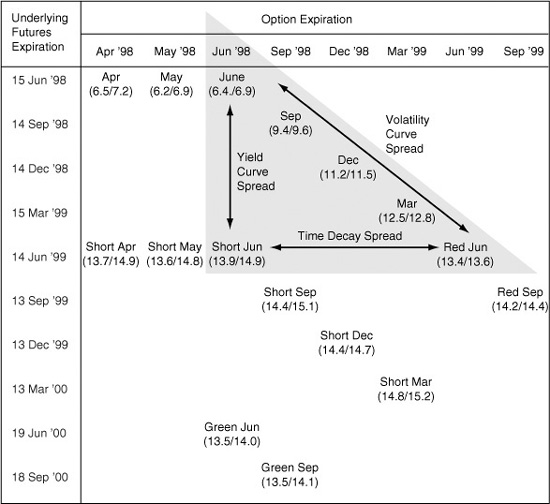
Eurodollar Strategy Triangle
The pivotal option for much of what professional traders are doing with these options is the “short June” option, an option that is based on the June ′99 futures contract but that expires in June ′98. This option creates a triangle of trading opportunities. You can, for example, use the June ′98 and short June options to trade the slope of the yield curve and take advantage of the term structure of Eurodollar volatilities. Or you can use the short June and red June options to take advantage of different rates of time decay in the two options. In addition, you can use options along the hypotenuse of the triangle to ride the Eurodollar volatility curve.
FOMC and Other Volatility Trades
Short-term serial options such as April ′98 and May ′98, both of which are on the June ′98 futures contract, provide excellent vehicles for trading short-term views on Federal Reserve policy. A number of traders are drawn to off-diagonal trades using short March (a March ′99 option on a March ′00 futures contract) and red September (a September ′99 option on a September ′99 futures contract) to produce long-term positions with an interesting mixture of gamma, vega, and theta.
Spreads against OTC Treasury Options
Mid-curves also make good spreading vehicles for OTC Treasury options. Changes in the underlying rates for the short June and green June mid-curves—the June ′99 and June ′00 futures rates, respectively—are highly correlated with changes in term Treasury yields on 2-year and 3-year notes. OTC Treasury options that expire in 1 to 3 months can be spread against corresponding mid-curves with comparable times to expiration.
LIFFE Joins the Crowd
The CME’s success with serial and mid-curve options has prompted LIFFE to adopt a similar approach. On May 15, 1998, LIFFE has joined the crowd by listing serial and quarterly mid-curve options on their 3-month money market contracts including the Euro, Euromark, Eurolira, and Short Sterling.
THE FULL CONSTELLATION OF EURODOLLAR OPTIONS
The Chicago Mercantile Exchange has been filling in a matrix of options on Eurodollar futures that provides a wealth of option-trading opportunities at the short end of the curve. The full range of choices is illustrated in Exhibit 23.1, which shows the option expirations from left to right across the top and the underlying futures expirations from top to bottom at the left.
Notice just how rich the set of choices is. In addition to the standard quarterly options, you have serial options and mid-curve options as well.
Standard Quarterly Options
There are six standard quarterly contract months listed on any given day. Each quarterly option expiration corresponds to the expiration of the underlying futures contract, so you have June ′98 options on the June ′98 futures contract, September ′98 options on the September ′98 futures contract, and so on out to September ′99.
Serial Options
Near-term gaps between quarterly options are filled by monthly serial options that expire before their underlying quarterly futures expire. Notice along the top row of Exhibit 23.1 that there are April ′98 and May ′98 options on the June ′98 futures contract. Unlike the June ′98 option on the June ′98 futures contract, which expires on a Monday morning along with its underlying futures contract, the serial options expire on Fridays and require you to make or take delivery of the underlying futures contract if the option is exercised. These are not cash-settled options.
Mid-curve Options
Six quarterly mid-curve options are currently available for trading. The unique thing about these options is that they expire 1 or 2 years before their underlying futures expire. For example, you can trade a June ′98 option for which the underlying is the June ′99 futures contract. This particular option is identified in Exhibit 23.1 as “short Jun,” the name by which it is known on the CME floor. Also notice that you can trade a June ′98 option on the June ′00 futures contract. This is a 2-year mid-curve option, identified in Exhibit 23.1 as “green Jun.” Thus, you have three options that expire in June ′98 with underlying futures contracts spread out at 1-year intervals along the futures rate curve. You also have short September and green September at this writing.
Serial 1-Year Mid-curve Options
The CME also lists hybrids of serial and mid-curve options. Notice, for example, that you can trade an April ′98 option on the June ′99 futures contract. This option is identified as “short Apr” in Exhibit 23.1. You also can trade the short May option, which is a May ′98 option on the June ′99 futures contract. Who knows? In time, the CME may list serial 2-year mid-curve options as well.
THE BEAUTY OF THIS DESIGN
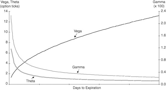
In the old days (the 1980s), you were limited mainly to trading Eurodollar options that expired at the same time as their underlying futures contracts. Thus, if you wanted to use these options to trade the slope of the short end of the futures curve, the trade would have an unusual mix of gamma, theta, and vega. As shown in Exhibit 23.2, short-dated options that are at or near the money are relatively rich in gamma and theta while relatively poor in vega. Thus, with a yield curve trade, you would necessarily be long (or short) gamma and short (or long) vega.
EXHIBIT 23.2
Vega, Gamma, and Theta
At-the-Money Call
The enlarged menu of Eurodollar contracts enables you to trade options expiring at the same (or nearly the same) time on different parts of the curve. The great thing about this arrangement is that you can use options with very similar gamma, theta, and vega characteristics to trade the slope of the yield curve.
As a bonus, you can trade options with different expirations on the same underlying futures contract. Thus, you can do some interesting volatility calendar trades that were not possible before.
THE EURODOLLAR STRATEGY TRIANGLE
To get an idea of how these trades work, consider three possibilities that lie along the sides of the highlighted triangle in Exhibit 23.1. One possibility, captured by June/short June along the left leg of the triangle, uses options with the same or nearly the same expirations on Eurodollar futures representing different parts of the curve. This is a yield curve trade with an interesting volatility spin. A second possibility, captured by short June/red June along the bottom leg of the triangle, uses options with different expirations but the same underlying futures contract. This kind of trade captures differences in time decay. A third possibility, captured by March/red June along the hypotenuse of the triangle, uses different expirations on different underlying futures to ride the volatility curve.
June/Short June (A Yield Curve Spread)
Suppose you think the yield curve is going to steepen. The June ′98 futures contract is trading at 94.33, which implies a rate of 5.67 percent. The June ′99 futures contract is trading at 94.18, which implies a rate of 5.82. The calendar spread is only 15 basis points and is trading near the low end of the range for the spread between the lead and the first “red” futures.
Instead of simply buying June ′98 futures and selling June ′99 futures, you might buy the 94.375 June ′98 call on the June ′98 futures contract and sell the 94.25 June ′98 call (known as “short June”) on the June ′99 futures contract.
One advantage of doing the trade with options is that you are usually buying a low-volatility option and selling a high-volatility option. This advantage appears in several forms. First, on March 25, you could do the trade at a 7-tick credit. For example, if you price the June ′98 call at a mid-market volatility of 6.7 percent, the price you pay is only 5 ticks. At the same time, if you price the short June call at a mid-market volatility of 14.4 percent, you find you could sell it for about 12 ticks.
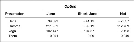
Second, as shown in Exhibit 23.3, you have a trade that gives you the appearance of positive gamma combined with positive theta. This highly peculiar situation is a direct result of the way volatility works on the options’ risk parameters. For options that are at or near the money, higher implied volatility produces lower gamma and higher theta. Vega, in contrast, is largely unrelated to the level of implied volatility. Because you are long the low-volatility option (the June option at 6.7 percent) and short the high-volatility option (the short June option at 14.4 percent), you have a position that is net long gamma that produces positive time decay for you as well. The positive gamma is partly an illusion, of course, because it works only with parallel shifts in the two underlying futures rates. (The higher volatility for the short June option suggests that non-parallel yield curve shifts are very likely.)
EXHIBIT 23.3
Risk Parameters of a Curve Steepener
Long 94.375 June ‘98 Call, Short 94.25 “Short June” ′98 Call
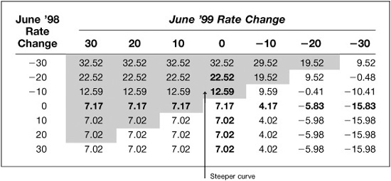
Whatever your views on the position’s net risk parameters, the higher volatility in the short June option gives you a nice cushion against a flattening of the curve and tips the odds in your favor overall. Exhibit 23.4 shows three futures rate curves—the current curve, the at-the-money curve, and the highest of the break-even curves. The current curve shows the 5.67 percent and 5.82 percent that correspond to market futures prices. The at-the-money curve shows the rates (5.625 percent and 5.75 percent) at which both options would expire exactly at the money. Notice that if the futures curve at expiration lies anywhere above the at-the-money curve, both options expire out of the money and you keep your 7-tick credit.
EXHIBIT 23.4
A Curve-Steepening Trade with Eurodollar Options Long 94.375 June ′98 Call, Short 94.25 “Short June” ′98 Call
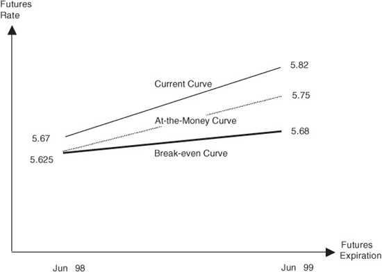
The break-even curve goes one step further and shows that the June ′99 rate could fall an additional 7 ticks to 5.68 percent before the loss on the short June option would rob you of your gain on the trade. As a result, the curve can actually flatten from its current slope of 15 basis points to 5.5 basis points before you stand to lose any money on the trade. (This break-even curve, by the way, is only the highest of the possible break-even curves. Any parallel curve that lies below this one also represents a break-even outcome.)
Your edge in the trade is reflected in the profit/loss summary shown in Exhibit 23.5, where all curve-steepening outcomes are shown in the upper left-hand part of the table. With parallel shifts in the curve, which are shown along the diagonal from the lower left corner to the upper right corner, you make 7 ticks or a little bit more. If both rates rise, you make at least 7 ticks because both options expire out of the money. If the curve actually steepens, you stand to make considerably more. Even if the curve flattens slightly, you can make money. If you contrast the 33-tick gain associated with a 60-basis-point steepening of the curve with the 16-tick loss associated with a 60-basis point flattening of the curve, the odds are, in a crude sense, 2-to-1 in your favor.
EXHIBIT 23.5
P/L of a Curve-Steepening Trade at Expiration Long 94.375 June ′98 Call, Short 94.25 “Short June” ′98 Call
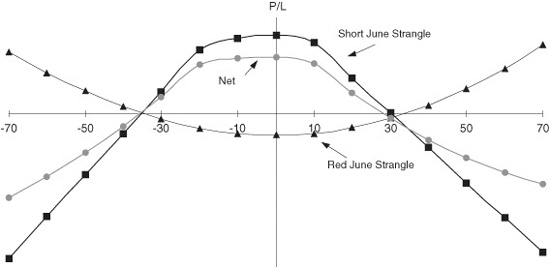
Short June/Red June (A Time Decay Spread)
Another possibility is to trade a calendar volatility spread based on the June ′99 futures contract. To do this, you have the June ′98 option on the June ′99 futures contract (known as short June), and the standard June ′99 option on the June ′99 futures contract (known as red June).
In this example, the implied volatilities at which the two options are trading are nearly the same, but the relative mixes of gamma, theta, and vega for the two options are very different. Short June options, which have roughly 3 months left to expiration, will have relatively high gammas and rates of time decay, while the red June options, which have nearly 15 months left to expiration, will have relatively high vegas. As a result, you might consider a delta-neutral position in which you sell a straddle or strangle using the short June options and buy a straddle or strangle using the red June options.
There is no single right way to construct this trade because of the different relative mixes of gamma, theta, and vega. Consider the way things look, however, if you sell 100 delta-neutral short June 94.00/94.25 strangles at a price of about 20 ticks per strangle and buy 100 delta-neutral red June strangles struck at the same prices for a price of about 56 ticks per strangle. Your net debit would be 3600 ticks [= 100 strangles × 36 ticks per strangle], and you would find yourself with a position that has negative gamma and positive theta (because the short June options have relatively more gamma and theta) and that has positive vega (because the red June options have relatively more vega). You can think of this trade, then, as a time decay spread that will benefit from an increase in implied volatility but that is exposed to the risk of too much actual or realized volatility.
A look at Exhibit 23.6 shows that your break-even on this position as of the expiration of the short June options on June 12, which is the Friday before the standard futures expiration, is roughly 30 basis points up or down.1 Thus, if you think that the June ′99 futures rate will change less than this, you will collect more time decay on the short June options than you pay on the red June options.
EXHIBIT 23.6
P/L for a Delta-Neutral Time Decay Spread
In the meantime, the position’s positive net vega is a potential bonus because of the comparatively low implied volatility at which you are buying the red June options. The term volatility in the short June option, which has 79 days to expiration, is 14.4 percent. The term volatility in the red June option, which has 446 days to expiration, is 13.5 percent. Since the underlying futures is the same for both of these options, this trade allows you to buy 1-year volatility roughly 2-1/2 months forward at 13.3 percent.2 If you view this as an exceptionally low level of implied volatility, you will welcome the positive vega that this trade affords.
March/Red June (A Volatility Curve Spread)
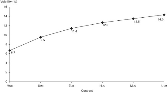
One well known feature of the Eurodollar volatility curve is that very short-dated futures rates exhibit quite a bit less volatility than do longer-dated futures rates. You can see this pattern in Exhibit 23.7, which shows the term structure of historical Eurodollar volatilities from the lead through the 6th contract. You can see the consequences of this pattern in Exhibit 23.8, which shows what the term structure of implied volatilities looked like on March 25 for the standard quarterly options on these futures contracts.
EXHIBIT 23.7
90-Day Historical Eurodollar Volatility A Cross-Sectional View
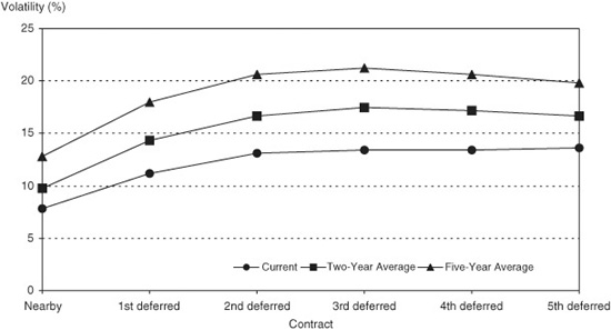
EXHIBIT 23.8
Term Structure of Implied Eurodollar Volatility
One way to profit from this pattern of volatilities is to “ride the Eurodollar volatility curve.” Under the right circumstances, you can do this by selling near-dated Eurodollar options and buying further-dated Eurodollar options. One might, for example, sell the March ′99 straddles on the March ′99 futures contract at 12.6 percent volatility and buy vega-equivalent June ′99 straddles on the June ′99 futures contract (red June) at 13.5 percent volatility. For example, you might sell 111 delta-neutral 94.25 March ′99 straddles for approximately 56 ticks per straddle and buy 100 of the red June 94.25 straddles at about 66 ticks per straddle for a net debit of 384 ticks [= 111 straddles × 56 ticks per straddle – 100 straddles × 66 ticks per straddle].
The resulting position would be vega-neutral, which sets you up to take advantage of a change in the implied volatility spread as the trade ages. In addition, you would earn net time decay on the position because you are short the higher theta option (and more of them). At the same time, you would be exposed to negative net gamma.
This is a trade that is put on for the comparatively long haul in the expectation that the implied volatility in the March options will fall faster than the implied volatility in the June options. For example, one might hold this position for 6 months to catch the steeper part of the volatility curve where the March ′99 straddles might be trading at 9.5 percent, while the June ′99 straddles (red June) might be trading at 11.4 percent. If so, you will have bought the spread at 0.9 percent [= 13.5 percent -12.6 percent] and sold it at 1.9 percent [= 11.4 percent -9.5 percent].
As long as there is no very great change in the March futures price, the trade can be expected to profit from a higher rate of time decay in the March options than would be paid on the long June options.
DIFFERENT VOLATILITY HORIZONS
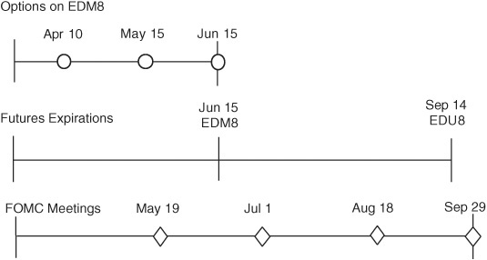
For traders who study the calendar of economic events for sources of volatility, serial option expirations on the same underlying futures contract provide a tool for trading the economic calendar. Adding a month to the life of an option generally sweeps in one more release of key economic information such as non-farm payroll, NAPM, and the CPI. Also, an additional month might bring with it an FOMC meeting or some other key economic event.
Consider Exhibit 23.9, which shows the schedule of FOMC meetings as it appeared on March 25. We can see that the June ′98 futures contract would be affected by any action the Fed takes on May 19 and by the market’s expectations about what the Fed might do at its meetings in July and August. What is interesting about the schedule, though, is that the April ′98 option on the June ′98 futures contract expires well before the May FOMC meeting, while the May ′98 option on the June ′98 futures contract expires on the Friday just before the FOMC meeting. As a result, anyone who believes that nothing will be revealed about the Fed’s intentions between March 25 and April 10 could sell April options and use the proceeds to buy May options and end up owning the May options cheap once the April options expire. Similarly, you might then sell May options and buy June options when you reach the high time decay part of the May option’s life.
EXHIBIT 23.9
Timeline of FOMC Meetings
MID-CURVE OPTIONS VERSUS OTC TREASURY OPTIONS
The mid-curve options such as short June and short September make it possible to trade the spread between Treasury yield volatility and Eurodollar volatility. Before the introduction of mid-curve options, anyone who wanted to trade Eurodollar options against OTC Treasury options was stuck with one or another of two mismatches. First, if you matched the expirations of the options, the underlying rates were only loosely correlated. Second, if you matched the correlations of the two underlying rates, the option expirations could be a year or more apart.
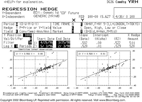
For example, the June ′98 option on the June ′98 Eurodollar contract would have roughly the same mix of gamma, theta, and vega as a 3-month OTC option on a 2-year Treasury note. But the June ′98 futures rate would be only loosely correlated with the spot or forward yield on a 2-year Treasury. Notice in Exhibit 23.10 that the lead Eurodollar rate changes only half a basis point for each basis point change in the on-the-run (OTR) Treasury yield and that the R2 (explanatory power) of the regression is only 0.52.
EXHIBIT 23.10
First Eurodollar Rate (Dependent) against OTR 2-Year Treasury Yield (Independent)
April 26, 1996−March 25, 1998; R2 = 0.52
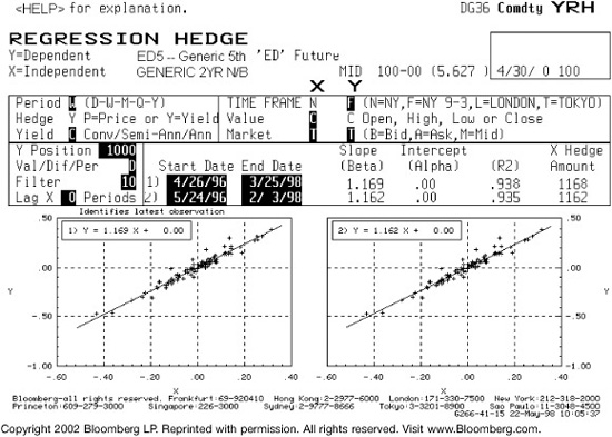
A better match for the yield on a 2-year Treasury, as shown in Exhibit 23.11, would be provided by something like the 5th Eurodollar contract rate, which in this case would be the June ′99 contract. This rate changes 1.17 basis points for each basis point change in the 2-year Treasury yield, and the R2 is 0.94. But the June ′99 option on the June ′99 futures contract would have altogether the wrong mix of gamma, theta, and vega for a spread against a shorter-dated OTC Treasury option.
EXHIBIT 23.11
Fifth Eurodollar Rate (Dependent) against OTR 2-Year Treasury Yield (Independent)
April 26, 1996−March 25, 1998; R2 = 0.94
Now that we have the mid-curve options, though, we can have the best of both worlds. The April ′98, May ′98, and June ′98 options on the June ′99 Eurodollar contract provide good gamma, theta, and vega matches for OTC 2-year Treasury options with roughly 1, 2, and 3 months to expiration.
Eurodollar/Treasury Volatility Spread Trading
The volatility of any given Eurodollar futures rate such as that implied by red June (that is, the June ′99 futures contract) can be thought of as comprising two parts: (1) the volatility of a corresponding forward Treasury rate, and (2) the volatility of the forward TED or swap spread. As such, the volatility of the Eurodollar rate will differ from that of a term Treasury yield for two reasons: (1) a less than perfect correlation between changes in the forward Treasury rate and the term Treasury yield, and (2) changes in the swap or TED spread.
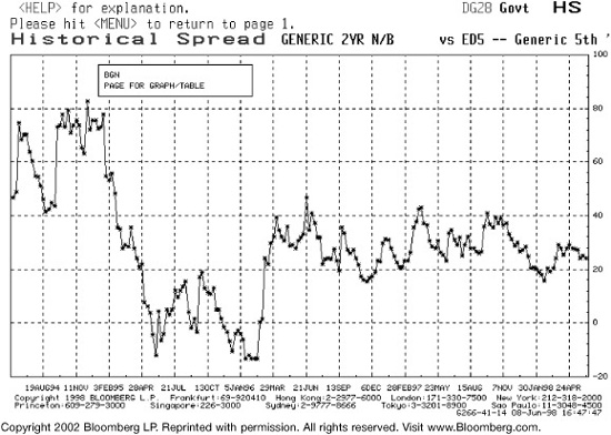
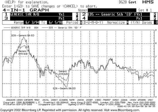
Thus, if you can buy Eurodollar volatility at a level that is roughly equivalent to term Treasury yield volatility, you can benefit both from the lack of perfect correlation between forward and term rates and from changes in the swap or TED spread. An idea of the day-to-day variability of the TED spread is provided in Exhibit 23.12, which shows the recent history of the 1-year and 2-year term TEDs. A recent history of the spread between the 5th Eurodollar rate and the on-the-run 2-year Treasury yield is provided in Exhibits 23.13 and 23.14.
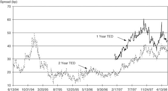
EXHIBIT 23.13
Yields of U.S. 5-Year Notes and 5th Eurodollar since June ′94
EXHIBIT 23.14
Yield Spread between 5-Year Notes and 5th Eurodollar since June ′94
In Basis Points
How Do You Compare the Volatilities?
Comparing implied volatilities in the two markets requires some care. First, the yield or rate levels are different. Second, the implied volatility quoted for an OTC Treasury option may be a forward yield volatility rather than a spot yield volatility.
Consider yield levels first. The June ′99 Eurodollar rate on March 25 was 5.82 percent and the mid-market implied volatility for the short June option was 14.4 percent. At these levels, the normalized or basis point volatility of the Eurodollar rate would be 0.838 or 83.8 basis points annualized [= 0.144 × 5.82]. If we use the regression coefficient of 1.17 from Exhibit 23.11, we find that the corresponding change in the spot Treasury yield would be 71.6 basis points [= 83.8/1.17], which would in turn represent a spot yield volatility of 12.9 percent [= 0.716/5.571, where 5.571 was the yield on the 5-1/2s of 3/00 on March 25]. As a result, any spot yield volatility above 12.9 percent would be rich relative to 14.4 percent Eurodollar volatility.
Forward yield volatilities tend to be higher than spot yield volatilities for two reasons. First, if repo rates do not change when Treasury note yields change, the change in the note’s forward price will be nearly the same as the change in the note’s spot price, but its forward DV01 is smaller than its spot DV01 so that the same price change translates into a larger yield change.
As a rule of thumb, you can convert a spot yield volatility into a forward yield volatility using the ratio of the note’s spot and forward months to expiration. For example, on March 25, the on-the-run Treasury had just over 23 months to expiration. One month later, it would have 22 months to expiration. Thus, a spot yield volatility of 12.9 percent would translate into a 1-month forward yield volatility of approximately 13.5 [= 12.9 × (23/22)] percent. A 2-month forward yield volatility would be 14.1 [= 12.9 × (23/21)] percent, and so forth. In practice, you would take care to refine these volatilities, but the rule of thumb gives you a quick and fairly reliable comparison.
How Do You Construct the Trades?
One advantage of trading in the over-the-counter options market is that you can choose your strikes and expirations to fit your circumstances. Thus, you can force the Treasury option expirations to line up with the Eurodollar option expirations. Moreover, you can choose your strikes to correspond to equivalent strikes in the Eurodollar market. For example, with the June ′99 Eurodollar rate at 5.82, you might trade strikes of 94.25 and 94.00, which correspond to rates of 5.75 and 6.00, which are 8 basis points below and 18 basis points above 5.82. If so, you could find appropriate strike prices for your Treasury options by finding the forward prices that correspond to yields that are about the same number of basis points above and below the current forward Treasury yield.
Once you have chosen your strikes, your last task is to find the appropriate amount of each option to do. Perhaps the easiest way to do this once one has lined up the expirations is to use the Eurodollar equivalent position of the Treasury note. If your OTC option were on $100 million of the on-the-run 2-year note and expires April 10, the Eurodollar hedge for the forward note exposure would be approximately 750 futures. Thus, the offsetting Eurodollar position would include 750 April ′98 options on the June ′99 futures contract. A May 15 option on the same note would require only 720 futures to hedge the forward note, and so you would do 720 of the May ′98 option on the June ′99 futures contract. A June option would require fewer still.
SOME THINGS TO KEEP IN MIND
Standard (non-mid-curve) serial options as well as serial and quarterly mid-curve options typically expire on the Friday before the expiration of standard quarterly options. For some strategies, such as the June-short June yield curve spread discussed above, this may entail slight expiration mismatches. Also, you must be prepared to make or take delivery of the underlying futures if these options are exercised, as they are not cash settled.
Strike prices for most Eurodollar options come in quarter point increments (e.g., 94.00, 94.25,…). In low-volatility environments this space between strikes can loom large. This is particularly true of options with relatively short times to expiration. Exhibit 23.8 showed that short-dated Eurodollar options can (and often do) have much lower implied volatilities than longer-lived contracts. Partly for this reason, the CME fills the spaces between some of the nearby contracts with so-called half-strikes, which come in 0.125 increments (e.g., 94.125, 94.25, 94.375,…). Every time a new quarterly option becomes the nearby option, half strikes are added for it and the subsequent two serial options. No additional contracts are given half strikes until the next quarterly contract becomes the nearby option, so the number of non-mid-curves with half strikes can range from one to three at any given time. The nearby 1-year mid-curve always has half strikes available.
LIFFE’s OPTIONS
On May 15, LIFFE added 1-year mid-curves to its Euro, Eurolira, Euromark, and Short Sterling options offerings. Two quarterly and two serial expiration months are currently available. Much like the initially tepid reception that first greeted Eurodollar mid-curves, these contracts have gotten off to a slow start. With all the things that can be done with these products, it seems unlikely that they will remain underutilized for long.