Computing Uniqueness Indices with PROC REG
When the SELECTION=RSQUARE option is included in the MODEL statement of PROC REG, it requests that all possible multiple regression equations be created, given the predictor variables that are specified in the MODEL statement. This means that it creates every possible regression equation that could be created by taking the predictors one at a time, every possible equation that could be created by taking the predictors two at a time, and so forth. The last equation it creates is the full equation: that which includes all predictor variables listed in the MODEL statement.
Output from this procedure reports only the R2 obtained for each of these equations (and not information concerning the regression coefficients, sum of squares, and so forth). The SELECTION=RSQUARE option is therefore useful for quickly and efficiently determining the percentage of variance in a criterion that is accounted for by every possible combination of predictor variables.
Although this information can be used for a number of purposes, this chapter shows how to use it to determine the uniqueness index for each predictor and how to test the significance of each uniqueness index. Earlier, it was said that the uniqueness index for a given predictor indicates the percentage of observed variance in the criterion that is accounted for by this predictor, over and above the variance accounted for by the other predictors. It can also be defined as the squared semipartial correlation between a criterion variable and the predictor variable of interest, after statistically controlling for the variance that the predictor shares with the other predictors.
Writing the Program
Here is the general form for the program statements that request the SELECTION=RSQUARE option with PROC REG:
PROC REG   DATA=dataset-name;
   MODEL  criterion  =  predictor-variables  /  SELECTION=RSQUARE;
RUN;
The names of the predictor variables in the MODEL statement should be separated by at least one space. The SELECTION=RSQUARE option computes and prints the R2 value for every possible regression equation that can be created from these variables. First, it will print R2 for a series of 1-predictor models, in which each predictor variable is the sole X variable in its own equation. Next, a series of 2-predictor models is printed in which the various equations represent every possible combination of predictors taken two at a time. The procedure continues in this manner until a single equation containing all of the predictor variables is printed.
These are the program statements that request the REG procedure for the current analysis. Notice that the MODEL statement is identical to that used with the previous REG procedure except that the STB option is replaced with the SELECTION=RSQUARE option:
PROC REG   DATA=D1;
   MODEL COMMIT = REWARD COST INVESTMENT ALTERNATIVES /
      SELECTION=RSQUARE;
RUN;
The results produced by these statements appear as Output 14.3.
Output 14.3. Results of the REG Procedure with the SELECTION=RSQUARE Option
                     The SAS System

                    The REG Procedure
                     Model: MODEL1
             Dependent Variable: COMMITMENT

                   R-Square Selection Method

Number in
  Model      R-Square     Variables in Model

       1       0.5184    ALTERNATIVES
       1       0.3770    INVESTMENT
       1       0.3317    REWARD
       1       0.0616    COST
-------------------------------------------------------------
       2       0.6248    INVESTMENT ALTERNATIVES
       2       0.5920    REWARD ALTERNATIVES
       2       0.5215    COST ALTERNATIVES
       2       0.4523    REWARD INVESTMENT
       2       0.4454    COST INVESTMENT
       2       0.3319    REWARD COST
-------------------------------------------------------------
       3       0.6436    REWARD INVESTMENT ALTERNATIVES
       3       0.6371    COST INVESTMENT ALTERNATIVES
       3       0.5947    REWARD COST ALTERNATIVES
       3       0.4690    REWARD COST INVESTMENT
-------------------------------------------------------------
4 0.6457 REWARD COST INVESTMENT ALTERNATIVES |
Interpreting the Results of PROC REG with SELECTION=RSQUARE
1. Make Sure That Everything Looks Right
In Output 14.3, the fourth line from the top indicates that the criterion variable is COMMITMENT, here referred to as the Dependent Variable.
The table of results created by the SELECTION=RSQUARE option includes three columns of information. The first column indicates the number of predictor variables included in a given multiple regression equation. The second column provides the R2 for that equation (i.e., the percent of variance in the criterion variable accounted for by this set of predictors). The third column specifies the names of the predictor variables included in each equation.
In the first section of this table (the section containing the 1-predictor models), you can see that the equation that includes only the predictor ALTERNATIVES has an R2 of approximately 0.52 (meaning that ALTERNATIVES account for approximately 52% of the variance in COMMITMENT). In the second section of the table (the section containing 2-predictor models), you can see that the model containing INVESTMENT and ALTERNATIVES account for about 62% of the variance in COMMITMENT.
2. Determine the Uniqueness Index for the Predictor Variables of Interest
The formula for determining the uniqueness index for a predictor variable is as follows:
U = R2Full – R2Reduced
where:
For example, assume that you want to determine the uniqueness index for the predictor, ALTERNATIVES. First, you identify the observed value of R2 for the full regression equation. This is the equation that contains all four predictors: REWARD; COST; INVESTMENT; and ALTERNATIVES. In Output 14.3, you first look under the heading “Variables in the Model” to find the single entry that contains the names of all four variables. This is the last entry on the page; under the heading “R-square,” you see that the R2 for this 4-variable model is approximately .65.
Next, you find the R2 for the reduced model: the model that includes all variables except for the variable of interest, ALTERNATIVES. Under “Variables in the Model,” you find the model containing only REWARD, COST, and INVESTMENT. To the left, the R2 for this model (the reduced model) is approximately .47. It is now possible to calculate the uniqueness index for ALTERNATIVES by inserting these values in the formula:
U = R2Full – R2Reduced
U = .65 – .47
U = .18
The uniqueness index for ALTERNATIVES is 0.18. There are several ways that this finding could be stated in a report; a few of these are now presented:
alternative value accounted for approximately 18% of the variance in commitment, beyond the variance accounted for by the other three predictor variables;
alternative value accounted for approximately 18% of the incremental variance in commitment;
the squared semi-partial correlation between alternative value and commitment was .18, while partialling variance that commitment shared with the other three predictors.
Once the uniqueness index is determined, it can be tested for statistical significance. This means testing the null hypothesis that the uniqueness index for the variable of interest is equal to zero. This can be done by using the formula for testing the significance of the difference between two R2 values. This formula is again reproduced here:

where:
| R2Full | = | The obtained value of R2 for the full multiple regression equation; that is, the equation containing the larger number of predictor variables. |
| R2Reduced | = | The obtained value of R2 for the reduced multiple regression equation; that is, the equation containing the smaller number of predictor variables. |
| KFull | = | The number of predictor variables in the full multiple regression equation. |
| KReduced | = | The number of predictor variables in the reduced multiple regression equation. |
| N | = | The total number of participants in the sample. |
Begin by testing the significance of the uniqueness index for ALTERNATIVES. Remember that the “full equation” in this analysis is the equation that contains all four predictor variables and produced an R2 of approximately .65. The “reduced equation” contains only three variables (all variables except ALTERNATIVES) and produced an R2 of approximately .47. These analyses were based on a sample of 48 responses. Here, these figures are paired with the appropriate symbols from the formula:
| R2Full | = .65 |
| R2Reduced | = .47 |
| KFull | = 4 |
| KReduced | = 3 |
| N | = 48 |
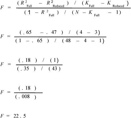
These values are now inserted in the appropriate locations in the formula, and the F ratio is calculated:

The obtained F for this test is 22.5. To determine whether this F is large enough to reject the null hypothesis, you must first find the critical value of F appropriate for the test. To do this, turn to the table of F values found in Appendix C in the back of this text. You need to locate the critical value of F that is appropriate when p = .05, and corresponds to the following degrees of freedom:
df for the numerator = KFull – KReduced
df for the denominator = N – KFull – 1
Notice that these degrees of freedom are already calculated in the preceding F formula: the df for the numerator (KFull – KReduced) is in the numerator of the F formula and the df for the denominator (N – KFull – 1) is in the denominator of the formula. There, it is determined that the df statistic for the numerator was 4 – 3 = 1, and the df statistic for the denominator was 48 – 4 – 1 = 43.
A table of F values shows that the critical value of F with 1 and 43 degrees of freedom is approximately 4.07 (p < .05). Your obtained F value of 22.5 is considerably larger than this critical value, so you can reject the null hypothesis that the uniqueness index is zero. Apparently, ALTERNATIVES account for a significant amount of variance in COMMITMENT in excess of the variance accounted for by the remaining X variables.
At this point, you would proceed to test the uniqueness index for each of the remaining X variables in the equation. In each case, calculating the uniqueness index for a given variable involves finding the percentage of variance in COMMITMENT that was accounted for by the equation excluding that predictor (from Output 14.3) and subtracting this value from the R2 value for the 4-variable model (.65). Here, the uniqueness index for each of the remaining three X variables is calculated:
| REWARD: | .65 – .64 = .01 |
| COST: | .65 – .64 = .01 |
| INVESTMENT: | .65 – .60 = .05 |
The preceding shows that REWARD accounts for approximately 1% of the variance in COMMITMENT, beyond the variance accounted for by the other three variables. The same is true for COST. INVESTMENT, on the other hand, has a somewhat larger uniqueness index, accounting for approximately 5% of the incremental variance in COMMITMENT.
Testing the statistical significance of the remaining three uniqueness indices is relatively straightforward because most of the necessary calculations have already been performed when testing the significance of ALTERNATIVES. Here, again, is the formula:

Notice that most of the components of this formula remain unchanged when you test the significance of the uniqueness index of a different predictor variable. For example, regardless of which predictor variable’s uniqueness index is being tested,
(KFull – KReduced) will be equal to 4 – 3 = 1.
(1 – R2Full)will be equal to 1 – .65 = .35.
N – KFull – 1) will be equal to 48 – 4 – 1 = 43.
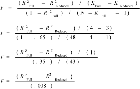
This means that the only component of the equation that will vary for different predictor variables is the quantity (R2Full – R2Reduced). Therefore, for the current regression equation, the F formula simplifies in the following way:

Remember that (R2Full – R2Reduced) is the formula for the uniqueness index for the variable of interest. Therefore, the preceding shows that, for the current regression equation, the F ratio that tests the significance of the uniqueness index for a given X variable can be calculated by dividing that uniqueness index by .008. The degrees of freedom for each of these tests will continue to be 1 and 43; this means that the critical value of F will continue to be 4.07.
You can now use this simplified formula to test the significance of the uniqueness indices for the remaining X variables.
For REWARD:

For COST:

For INVESTMENT:

Remember that, with 1 and 43 df, the critical value of F (p < .05) is 4.07 for each of these F tests. Only the obtained F ratio for INVESTMENT (at 6.25) exceeds this critical value. Therefore, only INVESTMENT demonstrates a statistically significant uniqueness index. These findings make sense when you consider the size of the uniqueness indices. INVEST accounts for approximately 5% of the unique variance in COMMITMENT, but REWARD and COST account for only 1%.
In summary, only ALTERNATIVES and INVESTMENT account for significant amounts of variance in COMMITMENT beyond the variance accounted for by the other predictors. ALTERNATIVES exhibits a uniqueness index of .18 while INVESTMENT demonstrates a uniqueness index of .05.
An earlier section of this chapter states that it is important to determine whether your linear combination of predictor variables accounts for a statistically significant amount of variance in the criterion, as well as whether this combination of predictors accounts for a meaningful (relatively large) amount of variance in the criterion. The same concerns remain when reviewing the results of these tests of the significance of uniqueness indices. With a large sample, it is possible to obtain a uniqueness index that is statistically significant even though the predictor variable accounts for negligible amounts of unique variance in the criterion (e.g., 2% and 3%). When reviewing your results, it is important to assess whether a significant uniqueness index is sufficiently large to be of substantive importance.
But how large is “large enough?” That depends, in part, on what prior research with your criterion variable has found. When doing research with a criterion variable that traditionally has been difficult to predict, a uniqueness index of .05 (and possibly even smaller) can be viewed as being of substantive importance. When researching a criterion that is relatively easy to predict, the uniqueness index might have to be larger to be considered important.
