An Example with Three Retained Components
The Questionnaire
The next example involves fictitious research that examines the investment model (Rusbult, 1980). As stated in earlier chapters, this model identifies variables believed to affect a person’s commitment to a romantic relationship. In this context, commitment refers to a person’s intention to maintain the relationship and stay with his/her current romantic partner.
One version of the investment model predicts that commitment is affected by three antecedent variables: satisfaction; investment size; and alternative value. Satisfaction refers to a participant’s affective response to the relationship. Among other things, participants report high levels of satisfaction when their current relationship comes close to their perceived ideal relationship. Investment size refers to the amount of time, energy, and personal resources that an individual has put into the relationship. For example, participants report high investments when they have spent a lot of time with their current partner and have developed mutual friends that might be lost if the relationship were to end. Finally, alternate value refers to the attractiveness of alternatives to one’s current partner. A participant would score high on alternate value if, for example, it would be appealing to date someone else or perhaps not to date at all.
Assume that you want to conduct research on the investment model and are in the process of preparing a 12-item questionnaire to assess levels of satisfaction, investment size, and alternate value in a group of participants involved in romantic relationships. Part of the instrument used to assess these constructs is reproduced here:
Indicate the extent to which you agree or disagree |
In the preceding questionnaire, items 1 through 4 were designed to assess satisfaction, items 5 through 8 were designed to assess investment size, and items 9 through 12 were designed to assess alternate value. Assume that you administer this questionnaire to 300 participants and now want to perform a principal component analysis on their responses.
Writing the Program
Earlier, it was mentioned that it is possible to perform a principal component analysis on a correlation matrix as well as on raw data (or covariance matrix). This section shows how the former is done. The following program enters the correlation matrix that provides all possible correlations between responses to the 12 items on the questionnaire, and performs a principal component analysis on these fictitious data:
 1     DATA D1(TYPE=CORR)  ;
 2        INPUT   _TYPE_    $
 3                _NAME_    $
 4                V1-V12    ;
 5     DATALINES;
 6     N     .    300  300  300  300  300  300  300  300  300  300  300  300
 7     STD   .   2.48 2.39 2.58 3.12 2.80 3.14 2.92 2.50 2.10 2.14 1.83 2.26
 8     CORR V1   1.00  .    .    .    .    .    .    .    .    .    .    .
 9     CORR V2    .69 1.00  .    .    .    .    .    .    .    .    .    .
10     CORR V3    .60  .79 1.00  .    .    .    .    .    .    .    .    .
11     CORR V4    .62  .47  .48 1.00  .    .    .    .    .    .    .    .
12     CORR V5    .03  .04  .16  .09 1.00  .    .    .    .    .    .    .
13     CORR V6    .05 -.04  .08  .05  .91 1.00  .    .    .    .    .    .
14     CORR V7    .14  .05  .06  .12  .82  .89 1.00  .    .    .    .    .
15     CORR V8    .23  .13  .16  .21  .70  .72  .82 1.00  .    .    .    .
16     CORR V9   -.17 -.07 -.04 -.05 -.33 -.26 -.38 -.45 1.00  .    .    .
17     CORR V10  -.10 -.08  .07  .15 -.16 -.20 -.27 -.34  .45 1.00  .    .
18     CORR V11  -.24 -.19 -.26 -.28 -.43 -.37 -.53 -.57  .60  .22 1.00  .
19     CORR V12  -.11 -.07  .07  .08 -.10 -.13 -.23 -.31  .44  .60  .26 1.00
20     ;
21
22     PROC FACTOR   DATA=D1
23                   METHOD=PRIN
24                   PRIORS=ONE
25                   MINEIGEN=1
26                   SCREE
27                   ROTATE=VARIMAX
28                   ROUND
29                   FLAG=.40   ;
30        VAR  V1-V12;
31     RUN;
The PROC FACTOR statement in this program follows the general form recommended for the initial analysis of a dataset. Notice that the MINEIGEN=1 statement requests that all components with eigenvalues greater than one be retained, and the SCREE option requests a scree plot of eigenvalues. These options are particularly helpful for the initial analysis of data as they can help determine the correct number of components to retain. If the scree test (or the other criteria) suggests retaining some number of components other than what would be retained using the MINEIGEN=1 option, that option can be dropped and replaced with the NFACT option.
Results of the Initial Analysis
The preceding program produced four pages of output, with the following information appearing on each page:
Page 1 includes the eigenvalue table.
Page 2 includes the scree plot of eigenvalues.
Page 3 includes the unrotated factor pattern and final communality estimates.
Page 4 includes the rotated factor pattern.
The eigenvalue table from this analysis appears on page 1 of Output 15.3. The eigenvalues themselves appear in the left-hand column under “Eigenvalue.” From these values, you can see that components 1, 2 and 3 provide eigenvalues of 4.47, 2.73, and 1.70, respectively. Furthermore, you can see that only these first three components provide eigenvalues greater than one. This means that three components are retained by the MINEIGEN criterion. Notice that the first nonretained component (component 4) displays an eigenvalue of approximately 0.85 which, of course, is well below 1.00. This is encouraging, as you have more confidence in the eigenvalue-one criterion when the solution does not contain “near-miss” eigenvalues (e.g., .98 or .99).
Output 15.3. Results of the Initial Principal Component Analysis of the Investment Model Data


The eigenvalue table in Output 15.3 also shows that the first three components combined account for approximately 74% of the total variance. (This variance value can be observed at the intersection of the column labeled “Cumulative” and row “3”.) According to the “percentage of variance accounted for” criterion, this once again suggests that it might be appropriate to retain three components.
The scree plot from this solution appears on page 2 of Output 15.3. This scree plot shows that there are several large breaks in the data following components 1, 2, and 3, and then the line begins to flatten beginning with component 4. The last large break appears after component 3, suggesting that only components 1 through 3 account for meaningful variance. This suggests that only these first three components should be retained and interpreted. Notice how it is almost possible to draw a straight line through components 4 to 12. The components that lie along a semi-straight line such as this are typically assumed to be measuring only trivial variance (i.e., components 4 through 12 constitute the “scree” of your scree plot).
So far, the results from the eigenvalue-one criterion, the variance accounted for criterion, and the scree plot are in accord to suggest that a three-component solution might be most appropriate. It is now time to review the rotated factor pattern to see if such a solution is interpretable. This matrix is presented on page 4 of Output 15.3.
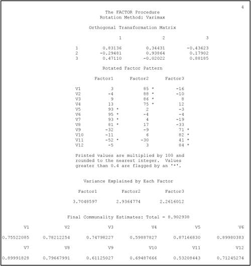
Following the guidelines provided earlier, you begin by looking for factorially complex items (i.e., items with meaningful loadings for more than one component). A review shows that item 11 (variable V11) is a complex item, loading on both components 1 and 3; item 11 should therefore be discarded. Except for this item, the solution is otherwise fairly straightforward.
To interpret component 1, you read down the column for FACTOR1 and see that items 5 through 8 exhibit significant loadings for this component. (Remember that item 11 has been discarded.) These items are shown here:
_____ 5. I have invested a great deal of time in my
current relationship.
_____ 6. I have invested a great deal of energy
|
All of these items pertain to the investments that participants have made in their relationships so it makes sense to label this the “investment size” component.
The rotated factor pattern shows that items 1 through 4 displayed meaningful loadings for component 2. These items are shown here:
_____ 1. I am satisfied with my current |
Given the content of the preceding items, it seems reasonable to label component 2 the “satisfaction” component.
Finally, component 3 displays large loadings for items 9, 10, and 12. (Again, remember that item 11 is discarded.) These items are shown here:
_____ 9. There are plenty of other attractive |
These items all seem to deal with the attractiveness of alternatives to one’s current relationship, so it makes sense to label this the “alternate value” component.
You can now step back and determine whether this solution satisfies the interpretability criteria presented earlier.
Are there at least three variables with meaningful loadings on each retained component?
Do the variables that load on a given component share the same conceptual meaning?
Do the variables that load on different components seem to be measuring different constructs?
Does the rotated factor pattern demonstrate “simple structure”?
In general, the answer to each of these questions is “yes,” indicating that the current solution is, in most respects, satisfactory. There is, however, a problem with item 11, which loads on both components 1 and 3. This problem prevented the current solution from demonstrating a perfectly “simple structure” (criterion 4 from above). To eliminate this problem, it might be desirable to repeat the analysis, this time analyzing all of the items except for item 11. This is done in the second analysis of the investment model data described below.
Results of the Second Analysis
To repeat the current analysis with item 11 deleted, it is necessary to modify only the VAR statement of the preceding program. This can be done by changing the VAR statement so that it appears as follows:
VAR V1-V10 V12;
All other aspects of the program remain as they were. The eigenvalue table, scree plot, the unrotated factor pattern, the rotated factor pattern, and final communality estimates obtained from this revised program appear in Output 15.4:
Output 15.4. Results of the Second Analysis of the Investment Model Data


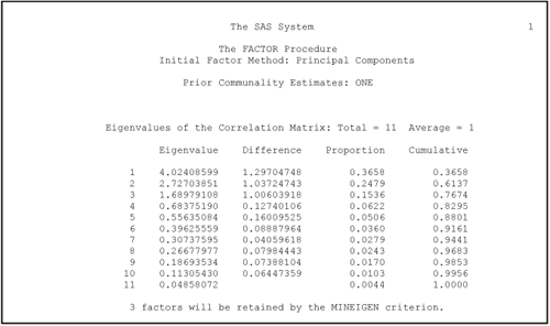
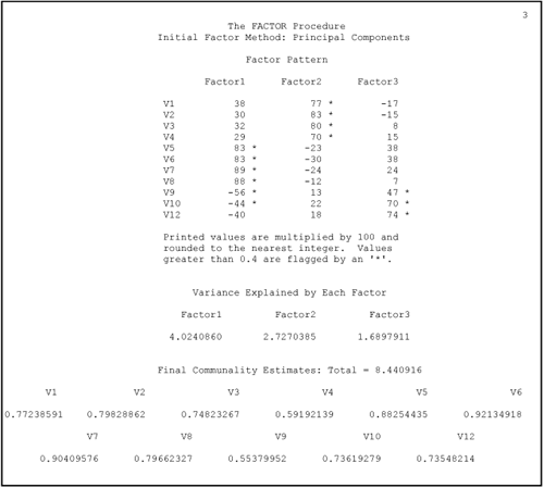
The results obtained when item 11 is deleted from the analysis are very similar to those obtained when it was included. The eigenvalue table of Output 15.4 shows that the eigenvalue-one criterion would again result in retaining three components. The first three components account for almost 77% of the total variance which means that three components would also be retained if you used the variance-accounted-for criterion. Also, the scree plot from page 2 of Output 15.4 is cleaner than had been observed with the initial analysis; the break between components 3 and 4 is now more distinct, and the eigenvalues again level off after this break. This means that three components would also be retained if the scree test were used to answer the number-of-components question.
The biggest change can be seen in the rotated factor pattern on page 4 of Output 15.4. The solution is now cleaner in the sense that no item now loads on more than one component (i.e., no complex items). The current results now demonstrate a somewhat simpler structure than had been demonstrated by the initial analysis of the investment model data.
