
The Paired-Samples t Test
Paired Samples versus Independent Samples
The paired-samples t test (sometimes referred to as the correlated-samples t test or matched-samples t test) is similar to the independent-samples test in that both procedures involve comparing two samples of observations, and determining whether or not the mean of one sample significantly differs from the mean of another. With the independent-samples procedure, the two groups of scores are completely independent (i.e., an observation in one sample is not related to any observation in the other). In experimental research, this is normally achieved by drawing a sample of participants and randomly assigning each to either a treatment or control condition. Because each participant contributes data under only one condition, the two samples are empirically independent.
With the paired-samples procedure, in contrast, each score in one sample is paired in some meaningful way with a score in the other sample. There are several ways that this can be achieved. The following examples illustrate some of the most commonly used approaches. One word of warning: the following fictitious studies merely illustrate paired sample designs, and do not necessarily represent sound research methodology from the perspective of internal or external validity. Problems with some of these designs are reviewed in a later section.
Examples of Paired-Samples Research Designs
Each Participant Is Exposed to Both Treatment Conditions
Earlier sections of this chapter described an analogue experiment in which level of reward was manipulated to see if it affected participants’ level of commitment to a romantic relationship. The procedure used in that study required participants to review 10 vignettes and then rate their commitment to each fictitious romantic partner. The dependent variable in the investigation was the rated amount of commitment that participants displayed toward partner 10. The independent variable was manipulated by varying the description of partner 10 that was provided to the participants; those in the “high-reward” condition read that partner 10 had several positive attributes while participants in the “low-reward” condition read that partner 10 did not have these attributes. This study was as an independent-samples study because each participant was assigned to either a high-reward condition or a low-reward condition, and no one was assigned to both.
This example could easily be modified to instead follow a paired-samples research design. You could do this by conducting the study with only one group of participants (rather than two), and having each participant rate partner 10 twice: once after reading the low-reward version of partner 10 and a second time after reading the high-reward version of partner 10.
It would be appropriate to analyze data derived from such a study using the paired-samples t test because it would be possible to meaningfully pair observations obtained under the two conditions. For example, participant 1’s rating of partner 10 under the low-reward condition could be paired with his or her rating of partner 10 under the high-reward condition, participant 2’s rating of partner 10 under the low-reward condition could be paired with his or her rating of partner 10 under the high-reward condition, and so forth. Table 8.1 shows how the resulting data could be arranged in tabular form:
| Commitment Ratings of Partner 10 | ||
|---|---|---|
| Participant | Low-Reward Condition | High-Reward Condition |
| Paul | 9 | 20 |
| Vilem | 9 | 22 |
| Pavel | 10 | 23 |
| Sunil | 11 | 23 |
| Maria | 12 | 24 |
| Fred | 12 | 25 |
| Jirka | 14 | 26 |
| Eduardo | 15 | 28 |
| Asher | 17 | 29 |
| Shirley | 19 | 31 |
Remember that your dependent variable is still the commitment ratings for partner 10. For participant 1 (Paul), you have obtained two scores on this dependent variable: a score of 9 obtained in the low-reward condition, and a score of 20 obtained in the high-reward condition. This is what it means to have the scores paired in a meaningful way: Paul’s score in the low-reward condition is paired with his score from the high-reward condition. The same is true for the remaining participants as well.
Participants Are Matched
The preceding study used a type of repeated measures approach: only one sample of participants participated; and repeated measurements on the dependent variable (commitment) were taken from each. That is, each participant contributed one score under the low-reward condition and a second score under the high-reward condition. A different approach could have used a type of matching procedure. With a matching procedure, a given participant provides data under only one experimental condition; however, each is matched with a different participant who provides data under the other experimental condition. The participants are matched on some variable that is expected to be related to the dependent variable, and matching is done prior to manipulation of the independent variable.
For example, imagine that it is possible to administer an “emotionality scale” to participants and that prior research has shown that scores on this scale are strongly correlated with scores on romantic commitment (i.e., the dependent variable in your study). You could administer this emotionality scale to 20 participants, and use their scores on the scale to match them; that is, to place them in pairs according to their similarity on the emotionality scale.
For example, scores on the emotionality scale might range from a low of 100 to a high of 500. Assume that John scores 111 on this scale, and Petr scores 112. Because their scores are very similar, you pair them together, and they become participant pair 1. Dov scores 150 on this scale and Lukas scores 149. Because their scores are very similar, you pair them together as participant pair 2. Table 8.2 shows how you could arrange these fictitious pairs of participants:
| Commitment Ratings of Partner 10 | ||
|---|---|---|
| Participant Pair | Low-Reward Condition | High-Reward Condition |
| Participant pair 1 (John and Petr) | 8 | 19 |
| Participant pair 2 (Dov and Lukas) | 9 | 21 |
| Participant pair 3 (Luis and Marco) | 10 | 21 |
| Participant pair 4 (Bjorn and Jorge) | 10 | 23 |
| Participant pair 5 (Ion and André) | 11 | 24 |
| Participant pair 6 (Martita and Kate) | 13 | 26 |
| Participant pair 7 (Blanche and Jane) | 14 | 27 |
| Participant pair 8 (Reuben and Joe) | 14 | 28 |
| Participant pair 9 (Mike and Otto) | 16 | 30 |
| Participant pair 10 (Sean and Seamus) | 18 | 32 |
Within each pair, one participant is randomly assigned to the low-reward condition and the other is assigned to the high-reward condition. Assume that, for each of the participant pairs in Table 8.2, the person listed first had been randomly assigned to the low condition and the person listed second had been assigned to the high condition. The study then proceeds in the usual way, with participants rating the various hypothetical partners.
Table 8.2 shows that John saw partner 10 in the low-reward condition and provided a commitment rating of 8. Petr saw partner 10 in the high-reward condition, and provided a commitment score of 19. When analyzing the data, you pair John’s score on the commitment variable with Petr’s score on commitment. The same will be true for the remaining participant pairs. A later section shows how to write a SAS program that does this.
When should the matching take place?Remember that participants are placed together in pairs on the basis of some matching variable before the independent variable is manipulated. They are not placed together in pairs on the basis of their scores on the dependent variable. In the present case, participants were paired based on the similarity of their scores on the emotionality scale. Later, the independent variable was manipulated and their commitment scores were recorded. Although they are not paired on the basis of their scores on the dependent variable, the researcher normally assumes that their scores on the dependent variable will be correlated. More on this in a later section. |
Pretest and Posttest Measures Are Taken
Consider now a different type of research problem. Assume that an educator believes that taking a foreign language course improves critical thinking among college students. To test this hypothesis, she administers a test of critical thinking to a single group of college students at two points in time. A pretest is administered at the beginning of the semester (prior to taking the language course), and a posttest is administered at the end of the semester (after completing the course). The data obtained from the two administrations appear in Table 8.3:
| Scores on Test of Critical Thinking Skills | ||
|---|---|---|
| Participant | Pretest | Posttest |
| Paul | 34 | 55 |
| Vilem | 35 | 49 |
| Pavel | 39 | 59 |
| Sunil | 41 | 63 |
| Maria | 43 | 62 |
| Fred | 44 | 68 |
| Jirka | 44 | 69 |
| Eduardo | 52 | 72 |
| Asher | 55 | 75 |
| Shirley | 57 | 78 |
You can analyze these data using the paired-samples t test because you can pair together the various scores in a meaningful way. That is, you can pair each participant’s score on the pretest with his or her score on the posttest. When the data are analyzed, the results will indicate whether or not there was a significant change in critical thinking scores over the course of the semester.
Problems with the Paired-Samples Approach
Some of the studies described in the preceding section utilize fairly weak experimental designs. This means that, even if you had conducted the studies, you might not have been able to draw firm conclusions from the results because alternate explanations could be offered for those results.
For example, consider the first study in which each participant was exposed to both the low-reward version of partner 10 as well as the high-reward version of partner 10. If you design this study poorly, it might suffer any of a number of confounds. For example, what if you designed the study so that each participant rated the low-reward version first and the high-reward version second? If you then analyzed the data and found that higher commitment ratings were observed for the high-reward condition, you would not know whether to attribute this finding to the manipulation of the independent variable (level of rewards) or to order effects (i.e., the possibility that the order in which the treatments were presented influenced scores on the dependent variable). For example, it is possible that participants tend to give higher ratings to partners that are rated later in serial order. If this is the case, the higher ratings observed for the high-reward partner might simply reflect such an order effect.
The third study described previously (which investigated the effects of a language course on critical thinking skills) also displays a weak experimental design: the single-group, pretest-posttest design. Assume that you administer the test of critical thinking to the students at the beginning and again at the end of the semester. Assume further that you observe a significant increase in their skill levels over this period. This would be consistent with your hypothesis that the foreign language course helps develop critical thinking.
Unfortunately, this would not be the only reasonable explanation for the findings. Perhaps the improvement was simply due to the process of maturation (i.e., changes that naturally take place as people age). Perhaps the change is simply due to the general effects of being in college, independent of the effects of the foreign language course. Because of the weak design used in this study, you will probably never be able to draw firm conclusions about what was really responsible for the students’ improvement.
This is not to argue that researchers should never obtain the type of data that can be analyzed using the paired-samples t test. For example, the second study described previously (the one using the matching procedure) was reasonably sound and might have provided interpretable results. The point here is that research involving paired-samples must be designed very carefully in order to avoid the problems discussed here. You can deal with most of these difficulties through the appropriate use of counterbalancing, control groups, and other strategies. Problems inherent in repeated measures and matching designs, along with the procedures that can be used to handle these problems, are discussed in Chapter 12, “One-Way ANOVA with One Repeated-Measures Factor,” and Chapter 13, “Factorial ANOVA with Repeated-Measures Factors and Between-Subjects Factors.”
When to Use the Paired-Samples Approach
When conducting a study that involves two treatment conditions, you will often have the choice of using either the independent-samples approach or the paired-samples approach. A number of considerations will influence your decision to use one design in place of the other. One of the most important considerations is the extent to which the paired-samples procedure results in a more sensitive test; that is, the extent to which the paired-samples approach makes it more likely to detect significant differences when they actually exist.
It is important to understand that the paired-samples t test has one important weakness when it comes to test sensitivity: the paired-samples test has only half the degrees of freedom as the equivalent independent-samples test. (A later section shows how to compute these degrees of freedom.) Because the paired-samples approach has fewer degrees of freedom, it must display a larger t value to attain statistical significance (compared to the independent-samples t test).
Then why use this approach? Because, under the right circumstances, the paired-samples approach results in a smaller standard error of the mean (the denominator in the formula used to compute the t statistic). Other factors held equal, a smaller standard error results in a more sensitive test.
However, there is a catch: the paired-samples approach will result in a smaller standard error only if scores on the two sets of observations are positively correlated. This concept is easiest to understand with reference to the pretest-posttest study described previously. Table 8.4 again reproduces the fictitious data obtained in this study:
| Scores on Test of Critical Thinking Skills | ||
|---|---|---|
| Participant | Pretest | Posttest |
| Paul | 34 | 55 |
| Vilem | 35 | 49 |
| Pavel | 39 | 59 |
| Sunil | 41 | 63 |
| Maria | 43 | 62 |
| Fred | 44 | 68 |
| Jirka | 44 | 69 |
| Eduardo | 52 | 72 |
| Asher | 55 | 75 |
| Shirley | 57 | 78 |
Notice that, in Table 8.4, scores on the pretest appear to be positively correlated with scores on the posttest. That is, participants who obtained relatively low scores on the pretest (such as Paul) also tended to obtain relatively low scores on the posttest. Similarly, participants who obtained relatively high scores on the pretest (such as Shirley) also tended to obtain relatively high scores on the posttest. Although the participants might have displayed a general improvement in critical thinking skills over the course of the semester, their ranking relative to one another remained relatively constant. Participants with the lowest scores at the beginning of the term still tended to have the lowest scores at the end of the term.
The situation described here is the type of situation that makes the paired-samples t test the optimal procedure. Because pretest scores are correlated with posttest scores, the paired-samples approach should yield a fairly sensitive test.
The same logic applies to the other studies described previously. For example, Table 8.5 again reproduces the data obtained from the study in which participants were assigned to pairs based on matching criteria:
| Commitment Ratings of Partner 10 | ||
|---|---|---|
| Participant Pair | Low-Reward Condition | High-Reward Condition |
| Participant pair 1 (John and Petr) | 8 | 19 |
| Participant pair 2 (Dov and Lukas) | 9 | 21 |
| Participant pair 3 (Luis and Marco) | 10 | 21 |
| Participant pair 4 (Bjorn and Jorge) | 10 | 23 |
| Participant pair 5 (Ion and André) | 11 | 24 |
| Participant pair 6 (Martita and Kate) | 13 | 26 |
| Participant pair 7 (Blanche and Jane) | 14 | 27 |
| Participant pair 8 (Reuben and Joe) | 14 | 28 |
| Participant pair 9 (Mike and Otto) | 16 | 30 |
| Participant pair 10 (Sean and Seamus) | 18 | 32 |
Again, there appears to be a correlation between scores obtained in the low-reward condition and those obtained in the high-reward condition. This is apparently because participants were first placed into pairs based on the similarity of their scores on the emotionality scale, and the emotionality scale is predictive of how participants respond to the commitment scale. For example, both John and Petr (pair 1) display relatively low scores on commitment, presumably because they both scored low on the emotionality scale that was initially used to match them. Similarly, both Sean and Seamus (participant pair 10) scored relatively high on commitment, presumably because they both scored high on emotionality.
This illustrates why it is so important to select relevant matching variables when using a matching procedure. There is a correlation between the two commitment variables above because (presumably) emotionality is related to commitment. If, instead, you had assigned participants to pairs based on some variable that is not related to commitment (e.g., participant shoe size), the two commitment variables would not be correlated and the paired-samples t test would not provide a more sensitive test. Under those circumstances, you would achieve more statistical power by, instead, using the independent-samples t test and capitalizing on the greater degrees of freedom.
Example: An Alternative Test of the Investment Model
The remainder of this chapter shows how to write SAS programs that perform paired-samples t tests and how to interpret the results. The first example is based on the first fictitious study described earlier, which examined the effect of levels of reward on commitment to a romantic relationship. The study included 10 participants who each rated partner 10 twice: once after reviewing the low-reward version of partner 10 and once after reviewing the high-reward version. Table 8.6 reproduces the data obtained from the participants:
| Commitment Ratings of Partner 10 | ||
|---|---|---|
| Participant | Low-Reward Condition | High-Reward Condition |
| Paul | 9 | 20 |
| Vilem | 9 | 22 |
| Pavel | 10 | 23 |
| Sunil | 11 | 23 |
| Maria | 12 | 24 |
| Fred | 12 | 25 |
| Jirka | 14 | 26 |
| Eduardo | 15 | 28 |
| Asher | 17 | 29 |
| Shirley | 19 | 31 |
These data were keyed according to the following format:
| Line | Column | Variable Name | Explanation |
|---|---|---|---|
| 1 | 1-2 | LOW | Commitment ratings obtained when participants rated the low-reward version of partner 10 |
| 3 | blank | ||
| 4-5 | HIGH | Commitment ratings obtained when participants rated the high-reward version of partner 10 |
Notice from the preceding format that no variable codes “group membership” or “treatment condition.” Instead, two variables include commitment ratings: one variable includes commitment ratings obtained when participants reviewed the low-reward version of partner 10; and the second includes commitment ratings obtained when participants reviewed the high-reward version.
The Difference Score Variable
A paired-samples t test is performed by creating a difference score variable, and determining whether the average difference score is significantly different from zero. If the average difference score is significantly different from zero, you can conclude that your independent variable has a significant effect on the dependent variable (assuming that the study was well-designed and that certain other conditions hold).
In the present study, this difference score variable is created by starting with participants’ commitment scores obtained in the high-reward condition and subtracting from the high-reward commitment score their commitment score obtained in the low-reward condition.
If a participant’s commitment score from the high-reward condition is approximately equal to his or her commitment score from the low-reward condition, the resulting difference score is approximately equal to zero. This suggests that the participant’s level of commitment was not affected by the level of reward manipulation. If none of the participants are affected by the manipulation (on average), then the average difference across participants should be approximately zero. Therefore, if the average difference score is not significantly different from zero, you will fail to reject the null hypothesis and will, instead, conclude that the manipulation had no effect on mean level of commitment.
On the other hand, assume that your manipulation does have the expected effect on commitment. This would mean that, for most participants, commitment ratings obtained under the high-reward condition would tend to be greater than commitment ratings under the low-reward condition. Subtracting low-reward commitment scores from high-reward commitment scores under these circumstances would tend to produce positive difference scores (rather than zero or negative difference scores). Therefore, if your manipulation has the predicted effect, the average difference score should be both positive and significantly different from zero. This is important to remember when you later review the results of your analyses.
The DATA Step
The following SAS program statements input the data from Table 8.6:
 1        DATA D1;
 2           INPUT   #1   @1   LOW   2.
 3                        @4   HIGH  2.   ;

 5        DATALINES;
 6         9 20
 7         9 22
 8        10 23
 9        11 23
10        12 24
11        12 25
12        14 26
13        15 28
14        17 29
15        19 31
16        ;
17       RUN;
Here is the general form for the SAS statements to perform a paired-samples t test:
PROC MEANS;
   VAR criterion-variable1 criterion-variable2;
RUN;

PROC TTEST   DATA=dataset name
             HO=comparison number
             ALPHA=alpha level;
   PAIRED criterion-variable1*criterion-variable2;
RUN;
In the preceding, criterion-variable1 and criterion-variable2 are the variables that include scores on the dependent variable under the two treatment conditions. In the present study, they correspond to the variables LOW and HIGH respectively.
PROC MEANS computes descriptive statistics for these variables. This allows you to check the data for possible errors in entering the data or writing the input statement. It also provides the means and standard deviations for both variables.
In the preceding general form, the PROC TTEST statement contains the following option:
H0=comparison-number
The “comparison-number” that appears in this option should be the mean difference score expected under the null hypothesis. In most cases when you perform a paired-sample t test, the mean difference score expected under the null hypothesis is zero. Therefore, you should generally use the following option when performing a paired-samples t test:
H0=0
Note that the “0” that appears in the preceding option “H0” is a zero (0) and is not an uppercase letter “O.” In addition, the “0” that appears to the right of the equals sign is also a zero and is not the uppercase letter “O.”
If you omit the H0 option from the PROC TTEST statement, the default comparison number is zero. This means that, in most cases, there is no harm in omitting this option.
The general form of the PROC TTEST statement also contains the following option:
ALPHA=confidence alpha-level
This ALPHA option allows you to specify the size of the confidence limits that you will estimate around the difference between means. Specifying ALPHA=0.01 produces 99% confidence limits, specifying ALPHA=0.05 produces 95% confidence limits, and specifying ALPHA=0.1 produces 90% confidence limits. Assume that in this analysis, you wish to create 95% confidence limits. This means that you will include the following option in the PROC TTEST statement:
ALPHA=0.05
The preceding general form also includes the following PAIRED statement:
PAIRED criterion-variable1*criterion-variable2;
In the PAIRED statement, you should list the names of the two SAS variables that contain the scores on the criterion variable obtained under the two treatment conditions. Notice that there is an asterisk (*) that separates the two variable names.
When SAS performs a paired-samples t test, it subtracts scores obtained under one condition from scores obtained under the other to create a new variable consisting of the difference scores. (This is done for you automatically.) The order in which you type your criterion variable names in the PAIRED statement determines how these difference scores are created. Specifically, SAS subtracts scores on criterion-variable2 from scores on criterion-variable1 in the example above. In other words, it subtracts scores on the variable on the right side of the asterisk from scores on the variable on the left side of the asterisk.
Actual SAS Statements for PROC TTEST
Below are the actual statements that request that SAS perform a paired-samples t test on the present data set.
PROC TTEST   DATA=D1   H0=0   ALPHA=.05;
   PAIRED   HIGH*LOW;
RUN;
In this PROC TTEST statement, you can see that you requested the option H0=0. This requests that SAS test the null hypothesis that the difference between the low- and high-reward conditions equals zero.
The PROC TTEST statement also includes the option ALPHA=0.05. This requests that SAS compute the 95% confidence interval for the difference between the means. (This is also the default alpha level, meaning that the SAS program computes the 95% confidence interval automatically even if not specifically requested.)
The PAIRED statement lists the SAS variable HIGH on the left side of the asterisk and LOW on the right. This means that scores on low-reward condition will be subtracted from scores on high-reward condition when computing difference scores. Given this format, if the mean difference score is a positive number, you will know that the participants displayed higher commitment scores under the high-reward condition than under the low-reward condition on average. Conversely, if the mean difference score is a negative number, you will know that participants displayed higher commitment scores under the low-reward condition than the high-reward condition.
The following is the entire program, including the DATA step, to analyze the fictitious data from Table 8.6. Notice how the actual variable names LOW and HIGH appear in the appropriate locations in lines 17 to 24.
 1        DATA D1;
 2           INPUT   #1   @1   LOW   2.
 3                        @4   HIGH  2.   ;
 4
 5        DATALINES;
 6         9 20
 7         9 22
 8        10 23
 9        11 23
10        12 24
11        12 25
12        14 26
13        15 28
14        17 29
15        19 31
16        ;
17        RUN;
18        PROC MEANS   DATA=D1;
19           VAR LOW HIGH;
20        RUN;
21
22        PROC TTEST   DATA=D1   H0=0   ALPHA=.05;
23           PAIRED HIGH*LOW;
24        RUN;
Interpreting the SAS Output
Output 8.3 presents the results obtained from the preceding program, both the PROC MEANS and PROC TTEST procedures. Review the results to first verify that everything ran as expected. Under the column headed “N,” you see that there were 10 observations for both variables. This is as expected, since there were 10 participants providing data under both conditions. Under the column headed “Mean,” you can see that the average commitment score in the low-reward condition was 12.8 while the average in the high-reward condition was 25.1. Participants therefore displayed higher levels of commitment for the high-reward version of partner 10, consistent with your hypothesis. (Later, you will determine whether these differences are statistically significant.)
Output 8.3. Results of the Paired-Samples t Test, Investment Model Study
                                The MEANS Procedure

  Variable     N            Mean         Std Dev         Minimum         Maximum
  ------------------------------------------------------------------------------
  LOW         10      12.8000000       3.3928028       9.0000000      19.0000000
  HIGH        10      25.1000000       3.4140234      20.0000000      31.0000000
  ------------------------------------------------------------------------------


                               The TTEST Procedure

                                   Statistics

               Lower CL          Upper CL  Lower CL           Upper CL
Difference   N     Mean    Mean      Mean   Std Dev  Std Dev  Std Dev    Std Err

HIGH - LOW  10   11.817    12.3    12.783    0.4643   0.6749   1.2322     0.2134


                                     T-Tests

                    Difference       DF    t Value     Pr > |t|

HIGH - LOW 9 57.63 <.0001 |
Earlier in the chapter, you learned that possible scores on the commitment scale can range from 4 to 36. You can now review the values in the “Minimum” and “Maximum” columns to verify that no observed values fell outside of this range. (Values exceeding these limits could indicate an error in entering the data or writing the input statement.) The output shows that observed scores on LOW range from 9 to 19 and that observed scores on HIGH range from 20 to 31. These values fall within your expected range, so there is no obvious evidence of errors. With this done, you are now free to review the output results relevant to your null hypothesis.
The bottom half of Output 8.3 provides the results produced by PROC TTEST. This section also provides results pertaining to the difference score between low- and high-reward conditions. In the middle section of the table, you can see that the average difference score was 12.3. This value is found in the column labeled “Mean” to the right along the row labeled “HIGH – LOW.” To determine whether this is in error, you can manually compute the difference between means and compare it against the mean difference core of 12.3. From the first section of the output, you can see that the mean score for the low-reward condition was 12.8 and the mean score for the high-reward condition was 25.1. Subtracting the former mean from the latter results in the following:
25.1 – 12.8 = 12.3
Therefore, you can see that using the means from PROC MEANS to compute the mean difference by hand results in the same difference as was reported in the output of PROC TTEST. Again, this suggests that there were no errors made when entering the data or when writing the SAS program itself.
This positive value indicates that, on the average, scores on HIGH tended to be higher than scores on LOW. The direction of this difference is consistent with your prediction that higher rewards are associated with greater levels of commitment.
Also presented in the middle of this table are the confidence limits for this mean difference. As you remember from earlier in this chapter, a confidence interval extends from a lower confidence limit to an upper confidence limit. To find the lower confidence limit for the current difference between means, look below the label “Lower CL Mean.” There, you can see that the lower confidence limit for the difference is 11.82. To find the upper confidence limit, look below the label “Upper CL Mean.” There, you can see that the upper confidence limit for the difference is 12.78. This means that you can estimate with a 95% probability that the actual difference between the mean of the low-reward condition and the mean of the high-reward condition in the population is somewhere between 11.82 and 12.78.
Notice that this interval does not contain the value of zero. This indicates that you can reject the null hypothesis (i.e., there is no difference between the low- and high-reward conditions).” If the null hypothesis were true, you would have expected the confidence interval to include a value of zero (i.e., a difference score of zero). The fact that your confidence interval does not contain a value of zero indicates rejection of the null hypothesis. To determine the level of statistical significance, review the t test results below in Output 8.3.
The t statistic in a paired-samples t test is computed using the following formula:

where:
| Md= | the mean difference score and; |
| SEd= | the standard error of the mean for the difference scores (the standard deviation of the sampling distribution of means of difference scores). |
The final section in Output 8.3 contains the relevant t statistic, under the heading “t Value”. This t value of 57.63 was obtained by dividing the mean difference score of 12.3 (under the heading “Mean”) by the standard error of the mean or .21 (under the heading “Std Err”). The t statistic had an associated p value less than . 01 (under the heading “Pr > |t|”). This p value is much lower than the standard cutoff of .05 indicating that the mean difference score of 12.3 was significantly different from zero. You can therefore reject the null hypothesis that the difference score is zero and can conclude that the mean commitment score of 25.1 observed with the high-reward version of partner 10 was significantly greater than the mean score of 12.8 observed with low-reward version of partner 10. In other words, you can tentatively conclude that the level of reward manipulation had an effect on rated commitment.
The degrees of freedom associated with this t test are equal to N–1, where N = the number of pairs of observations in the study. This is analogous to stating that N is equal to the number of difference scores that are analyzed. If the study involves taking repeated measures from a single sample, N equals the number of participants. However, if the study involves two sets of participants who are matched to form participant pairs, N will equal the number of participant pairs (i.e., half the total number of participants).
The present study involved taking repeated measures from a single sample of 10 participants. Therefore, N = 10 in this study, and the degrees of freedom are equal to 10 –1, or 9. This value appears below the heading “DF” in output 8.3.
Earlier in this chapter, you learned that an effect size can be defined as the degree to which a mean score obtained under one condition differs from the mean score obtained under a second. The symbol for effect size is d. When performing a paired-samples t test, the formula for effect size is as follows:
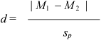
where:
| M1 = | the observed mean of the sample of scores obtained under Condition 1; |
| M2 = | the observed mean of the sample of scores obtained under Condition 2 and; |
| sp = | the estimated standard deviation of the population of difference scores. |
Although SAS does not automatically compute effect sizes, you can easily do so yourself using the information that appears in the output of PROC MEANS and PROC TTEST. First, you need the mean commitment level scores for both treatment conditions. These means appear in the upper section of Output 8.3.
In the preceding formula, M1 represents the observed sample mean for scores obtained under Condition 1 (low-reward condition). In Output 8.3, you can see that the mean commitment score for these participants was 12.8. In the preceding formula, M2 represents the observed mean obtained under Condition 2 (high-reward condition). You can see that the mean commitment score obtained under this condition was 25.1. Substituting these two means in the formula results in the following:

In the formula for d, Sp represents the estimated standard deviation of difference scores. This statistic appears in the “Statistics” table from the results of PROC TTEST. The estimated standard deviation of difference scores appears below the heading “Std Dev.” For the current study, you can see that this standard deviation is .67. Substituting this value in the formula results in the following:

Thus, the obtained index of effect size for the current study is 18.36. This means that the mean commitment score obtained under the low-reward condition differs from the mean commitment score obtained under the high-reward condition by 18.36 standard deviations. To determine whether this is a large or small difference, refer back to the guidelines provided by Cohen (1992) in Table 8.1. Your obtained d statistic of 18.36 is larger than the “large effect” value of .80. This means that the manipulation in your study produced a very large effect.
Summarizing the Results of the Analysis
You could summarize the results of the present analysis following the same format used with the independent groups t test as presented earlier in this chapter (e.g., statement of the problem, nature of the variables). Figure 8.5 illustrates the mean commitment scores obtained under the two conditions manipulated in the present study:
Figure 8.5. Mean Levels of Commitment Observed for Participants in High-Reward versus Low-Reward Conditions, Paired-Samples Design

You could describe the results of the analysis in a paper in the following way:
Results were analyzed using a paired-samples t test. This analysis revealed a significant difference between mean levels of commitment observed in the two conditions, t(9) = 57.63; p < .01. The sample means are displayed in Figure 8.4, which shows that mean commitment scores were significantly higher in the high-reward condition (M = 25.1, SD = 3.41) than in the low-reward condition (M = 12.8, SD = 3.39). The observed difference between these mean scores was 12.3 and the 95% confidence interval for the difference between means extended from 11.82 to 12.78. The effect size was computed as d = 18.36. According to Cohen's (1992) guidelines for t tests, this represents a very large effect.
Example: A Pretest-Posttest Study
An earlier section presented the hypothesis that taking a foreign language course will lead to an improvement in critical thinking among college students. To test this hypothesis, assume that you conducted a study in which a single group of college students took a test of critical thinking skills both before and after completing a semester-long foreign language course. The first administration of the test constituted the study’s pretest, and the second administration constituted the posttest. Table 8.7 again reproduces the data obtained in the study:
| Scores on Test of Critical Thinking Skills | ||
|---|---|---|
| Participant | Pretest | Posttest |
| Paul | 34 | 55 |
| Vilem | 35 | 49 |
| Pavel | 39 | 59 |
| Sunil | 41 | 63 |
| Maria | 43 | 62 |
| Fred | 44 | 68 |
| Jirka | 44 | 69 |
| Eduardo | 52 | 72 |
| Asher | 55 | 75 |
| Shirley | 57 | 78 |
You could enter the data for this study according to the following format:
| Line | Column | Variable Name | Explanation |
|---|---|---|---|
| 1 | 1-2 | PRETEST | Scores on the test of critical thinking obtained at the first administration |
| 3 | blank | ||
| 4-5 | POSTTEST | Scores on the test of critical thinking obtained at the second administration |
Here is the general form for the PROC MEANS and PROC TTEST statements to perform a paired-samples t test using data obtained from a study using a pretest-posttest design:
PROC MEANS;
   VAR pretest posttest;
RUN;

PROC TTEST   DATA=dataset name
             H0=comparison number
             ALPHA=alpha level;
   PAIRED posttest*pretest;
RUN;
Notice that these statements are identical to the general form statements presented earlier in this chapter, except that the “pretest” and “posttest” variables have been substituted for “variable1” and “variable2,” respectively.
The following is the entire SAS program to input the data from Table 8.7 and perform a paired-samples t test.
 1        DATA D1;
 2           INPUT   #1   @1   PRETEST   2.
 3                        @4   POSTTEST  2.   ;
 4
 5        DATALINES;
 6        34 55
 7        35 49
 8        39 59
 9        41 63
10        43 62
11        44 68
12        44 69
13        52 72
14        55 75
15        57 78
16        ;
17        RUN;
18
19        PROC MEANS   DATA=D1;
20           VAR PRETEST POSTTEST;
21        RUN;
22
23        PROC TTEST   DATA=D1
24             H0=0
25             ALPHA=.05;
26             PAIRED POSTTEST*PRETEST;
27        RUN;
The preceding program results in the analysis of two variables: PRETEST (each participant’s score on the pretest) and POSTTEST (each participant’s score on the posttest). Once again, a difference variable was created by subtracting each participant’s score on PRETEST from his or her POSTTEST score. Given the way that difference scores were created in the preceding program, a positive mean difference score would indicate that the average posttest score was higher than the average pretest score. Such a finding would be consistent with your hypothesis that the foreign language course would cause an improvement in critical thinking. If the average difference score is not significantly different from zero, however, your hypothesis would receive no support. (Again, remember that any results obtained from the present study would be difficult to interpret given the lack of an appropriate control group.)
You can interpret the results from the preceding program in the same manner as with Example 1, earlier. In the interest of space, those results do not appear again here.