
Chapter 3
Identifying Calcium Binding Sites in Proteins
3.1 Introduction
The number of experimentally and computationally derived structural models available in databases has been steadily increasing with the emergence of structural genomics projects worldwide. One important problem in current biology and chemistry is to assign proteins with functions based on 3D structure. Calcium, one of the most important metals for life, is responsible for regulating many biological processes through its interactions with numerous calcium binding proteins in different biological environments [1, 2]. Identifying the calcium binding sites is not only critical for the study of individual proteins but also helpful for revealing the general factors involved in such as the mechanisms governing calcium binding affinity, metal selectivity, and calcium-induced conformation change [3]. Sites are defined by a 3D location and a local neighborhood with a common structural or functional role. Non-calcium-binding sites are locations where the function does not occur or a different function is present. According to structural features, calcium binding sites can be classified as continuous or discontinuous [4, 5]. Continuous calcium binding sites consist of amino acids adjacent in primary sequence, usually in a highly conserved loop flanked by the helix–loop–helix, whereas discontinuous calcium binding sites consist of residues that are spatially proximate in the folded structure but distant in the sequence, and do not have conserved calcium binding loops and flanked helices.
Identification of the calcium binding sites in proteins is one of the main barriers to understanding the role of calcium in biological systems. Numerous efforts have been devoted to predicting and visualizing calcium binding sites in proteins with high accuracy and speed. Yamashita and coworkers [6] reported that metal ions bind at centers of high hydrophobicity contrast, which was further embedded within a shell of carbon-containing hydrophobic atom groups. They embedded the whole protein structure into a 3D grid and measured hydrophobicity contrast at each gridpoint in order to predict metal binding sites on the basis of this observation. Nayal and Di Cera [7] applied a similar approach to improve performance through replacing the contrast function with valence function with a clear cutoff between calcium binding and non-calcium-binding sites (nonsites). The computational calculations of both grid algorithms are intensive and thus not suitable for predicting calcium binding sites in proteins with required speed and accuracy. Several methods, such as FEATURE, protein seqFEATURE, or MetSite [8–15], used statistical approaches for recognizing calcium binding sites based on a variety of physical and chemical features in calcium binding sites and nonsites. Rychlewski et al. [15] illustrated the capability of predicting the precise locations of calcium binding sites with high coordination numbers based on the Fold-X empirical forcefield. However, the success rate of their results is low.
To overcome the disadvantages of the abovemeintioned approaches, we illustrate three methods based on the geometric and other key features of calcium binding sites in this chapter. The first method, called GG [16], applied a graph theory algorithm by taking advantage of its capability of extracting key features of the system [17, 18]. GG has obtained high performance with ![]() site sensitivity and 80% site selectivity, and more than 95% of the sites with four or more ligands have been accurately identified within 1 Å of the documented calcium ions. Their results have demonstrated that a cluster of four or more oxygen atoms has a high potential for calcium binding. The second method named as GG2.0 is an enhanced version of the GG method to predict calcium binding sites in proteins [19]. GG2.0 applies the maximal clique algorithm to find biggest local oxygen clusters and calculate the geometric filter related to the ratio between the size of the first shell and the second shell of calcium binding sites by using an optimization tool. Their results not only achieve the high performance of 98% site sensitivity and 86% site selectivity but also demonstrate that some oxygen clusters satisfying geometric criteria are not calcium binding sites with some fixed residue combinations. GSVM [20], a supervised classification model, is built by absorbing the advantages of statistical approaches and graph theory algorithm. On the basis of the maximal oxygen clusters, a putative calcium center (PCC) is located by minimizing the average distance between PCC and every oxygen atom for one maximal cluster. Spherical regions centered on PCC are chosen as putative calcium binding sites. GSVM distinguish between calcium binding sites and non-calcium-binding sites by taking spatial distribution of biophysical and biochemical properties as an input variable for a binary classification task. High performance with site sensitivity and site selectivity has been obtained through GSVM.
site sensitivity and 80% site selectivity, and more than 95% of the sites with four or more ligands have been accurately identified within 1 Å of the documented calcium ions. Their results have demonstrated that a cluster of four or more oxygen atoms has a high potential for calcium binding. The second method named as GG2.0 is an enhanced version of the GG method to predict calcium binding sites in proteins [19]. GG2.0 applies the maximal clique algorithm to find biggest local oxygen clusters and calculate the geometric filter related to the ratio between the size of the first shell and the second shell of calcium binding sites by using an optimization tool. Their results not only achieve the high performance of 98% site sensitivity and 86% site selectivity but also demonstrate that some oxygen clusters satisfying geometric criteria are not calcium binding sites with some fixed residue combinations. GSVM [20], a supervised classification model, is built by absorbing the advantages of statistical approaches and graph theory algorithm. On the basis of the maximal oxygen clusters, a putative calcium center (PCC) is located by minimizing the average distance between PCC and every oxygen atom for one maximal cluster. Spherical regions centered on PCC are chosen as putative calcium binding sites. GSVM distinguish between calcium binding sites and non-calcium-binding sites by taking spatial distribution of biophysical and biochemical properties as an input variable for a binary classification task. High performance with site sensitivity and site selectivity has been obtained through GSVM.
The rest of the chapter is organized as follows: Section 3.2 illustrates datasets, performance measurement, and detailed implementation of three methods: GG, GG2.0, and GSVM. Experimental results and discussion are presented in Section 3.3. Conclusions are included in Section 3.4.
3.2 Methods
3.2.1 Datasets
To compare these three methods with previous finding, we select a total of 123 proteins and 231 calcium binding sites in three datasets, which are queried from the metalloprotein database and browser (MDB) with the conditions that every calcium binding protein structure from PDB has resolution of ![]() Å from X-ray crystallography, each site has a coordination number of
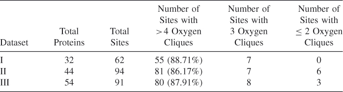
Å from X-ray crystallography, each site has a coordination number of ![]() , excluding water oxygen, and the PDB entry must be in the PDBSELECT nonhomology list. Nayal-Di Cera's 7 dataset (dataset I) contains 32 proteins with 62 calcium binding sites. Dataset II from Pidcock and Moore 5 has 44 proteins and 94 calcium binding sites, which are obtained from 515 fully normalized crystal structures of calcium binding proteins deposited in PDB from 1994 to 1998 with a resolution ranging from 1.0 to 2.5 Å. Liang's dataset (dataset III) contains 91 calcium binding sites from 54 proteins, and 14 non-calcium-binding proteins. These datasets are summarized in Table 3.1.
, excluding water oxygen, and the PDB entry must be in the PDBSELECT nonhomology list. Nayal-Di Cera's 7 dataset (dataset I) contains 32 proteins with 62 calcium binding sites. Dataset II from Pidcock and Moore 5 has 44 proteins and 94 calcium binding sites, which are obtained from 515 fully normalized crystal structures of calcium binding proteins deposited in PDB from 1994 to 1998 with a resolution ranging from 1.0 to 2.5 Å. Liang's dataset (dataset III) contains 91 calcium binding sites from 54 proteins, and 14 non-calcium-binding proteins. These datasets are summarized in Table 3.1.
Table 3.1 Description of Three Datasets (Ca−O ≤ 3.5 Å)
3.2.2 Performance Measurement
A qualified clique is a true prediction (TP) if its putative of calcium ion location falls into the cutoff distance (3.5 Å in our studies) from a documented calcium ion in a crystal structure. A documented calcium binding site is a true prediction site (TPS) if there is any prediction within the cutoff distance from this site. The performance of our studies are evaluated by site sensitivity (SEN) and site selectivity (SEL), which represent the percentage of TPS in the total sites and the percentage of TP in the total predictions, respectively.
3.2.3 GG Algorithm
3.2.3.1 Graph Algorithm
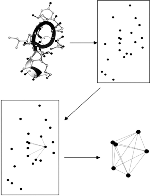
For a given protein structure as shown in Figure 3.1, the coordinates in the PDB file of oxygen atoms are extracted first. The distances between every two oxygen atoms are calculated. A graph ![]() is constructed accordingly, in which
is constructed accordingly, in which ![]() is the set of all oxygen atoms and each edge in
is the set of all oxygen atoms and each edge in ![]() exists between a pair of oxygen atoms apart within an O
exists between a pair of oxygen atoms apart within an O![]() O cutoff distance (6.0 Å in GG algorithm 17). The graph construction uses
O cutoff distance (6.0 Å in GG algorithm 17). The graph construction uses ![]() , where
, where ![]() is the number of oxygen atoms. A clique
is the number of oxygen atoms. A clique ![]() is a subset of
is a subset of ![]() such that every two vertices of
such that every two vertices of ![]() are connected by an edge. The number of vertices in the clique is defined as the size of a clique.
are connected by an edge. The number of vertices in the clique is defined as the size of a clique.
Figure 3.1 The schematic model of a GG program is shown. The oxygen atom positions (dark dots) are extracted from the protein structure, while the other atoms (light dots) are excluded. The distances between two oxygen atoms are calculated and an edge is assigned if the distance is below a cutoff distance (O![]() O cutoff). A potential calcium binding position is a clique (bottom right), which is a group in which every oxygen atom is linked to all other members of the group by edges.
O cutoff). A potential calcium binding position is a clique (bottom right), which is a group in which every oxygen atom is linked to all other members of the group by edges.
Instead of exhaustive search in grid methods, we use a backtracking algorithm to find cliques of certain sizes in ![]() . The time complexity of GG is linear because of the specificity of the graph
. The time complexity of GG is linear because of the specificity of the graph ![]() construction from a protein structure. Further more, the number of cliques is far less than the number of the gridpoints. Therefore, GG is more computational efficient compared with the previous methods. The pseudocode for finding cliques of four vertices in
construction from a protein structure. Further more, the number of cliques is far less than the number of the gridpoints. Therefore, GG is more computational efficient compared with the previous methods. The pseudocode for finding cliques of four vertices in ![]() is shown as Figure 3.2.
is shown as Figure 3.2.
1. Loop through all vertices a in V
2.   Loop through all vertices b in the adjacecy list of a
3.   output V:=V-{a} if no such b exists
4.     Loop through all vertices c adjacent to both a and b
5.     output V:=V-{a} if no such c exists
6.      Loop through all vertices d adjacent to both a, b, and c
7.        output clique {a,b,c,d}
8.      output V:=V-{a} if no such d exists
Figure 3.2 Pseudocode of the GG algorithm for finding all cliques of size 4.
3.2.3.2 Geometry Algorithm
The point that has the same distance to the four vertices of a clique is defined as the circumcenter (CC). The distance between CC and vertices of a clique is called psdCa![]() O. In order to eliminate false positives, a clique is considered as a putative calcium binding site only if psdCa
O. In order to eliminate false positives, a clique is considered as a putative calcium binding site only if psdCa![]() O falls into the range (
O falls into the range (![]() ), where
), where ![]() and
and ![]() are the lower and upper limits, respectively. Since the space for calcium binding should not be occupied by other atoms, GG algorithm further applied a D-filter to eliminate any cliques that contain nonoxygen atoms within a short distance (D-filter) from the CC. The complexity of this step algorithm is
are the lower and upper limits, respectively. Since the space for calcium binding should not be occupied by other atoms, GG algorithm further applied a D-filter to eliminate any cliques that contain nonoxygen atoms within a short distance (D-filter) from the CC. The complexity of this step algorithm is ![]() , where
, where ![]() is the number of all atoms other than oxygen. Dataset I was used to optimize the parameters such as psdCa
is the number of all atoms other than oxygen. Dataset I was used to optimize the parameters such as psdCa![]() O range and D-filter in order to achieve high accuracy and speed. By using an O
O range and D-filter in order to achieve high accuracy and speed. By using an O![]() O cutoff of 6.0 Å, a psdCa
O cutoff of 6.0 Å, a psdCa![]() O range of 1.8–3.0 Å and a D-filter equal to the psdCa
O range of 1.8–3.0 Å and a D-filter equal to the psdCa![]() O, the best performance was obtained.
O, the best performance was obtained.
3.2.3.3 Removal of Redundant Predictions
A merging algorithm was adopted to remove redundant predictions in one location. All putative sites in a protein are input in a vector and sorted by psdCa![]() O. The putative sites within 3.5 Å (center–center distance) from it are deleted once the one with the shortest psdCa
O. The putative sites within 3.5 Å (center–center distance) from it are deleted once the one with the shortest psdCa![]() O is determined. The merging procedure is repeated until the vector is empty. The computational complexity is not larger than
O is determined. The merging procedure is repeated until the vector is empty. The computational complexity is not larger than ![]() because it depends on the number of total comparisons.
because it depends on the number of total comparisons.
3.2.3.4 Computational Complexity Analysis
The computational complexity of GG is ![]() from the three steps of this algorithm, which can be simplified to
from the three steps of this algorithm, which can be simplified to ![]() because it is the dominant component.
because it is the dominant component.
3.2.4 GG2.0 Algorithm [19]
3.2.4.1 A Geometric Criterion
After oxygen cliques are found by using a graph algorithm similar to GG17, a carbon cluster around every oxygen cluster is also obtained because each oxygen atom is connected to one carbon atom. The least variance point (LVP) is defined as the geometric point that has a smallest variance with respect to every other atom/vertex of the cluster/clique. There exists a corresponding carbon cluster surrounding every oxygen cluster. These two clusters are thus called twin clusters, and the LVP of the oxygen cluster is chosen as the center of the twin clusters. The optimization function of fminsearch in the Matlab software was used to obtain the coordinates of the LVP of a cluster. Then the radius of oxygen/carbon cluster (RO/RC) can be calculated as
where and are the distances between the LVP and each oxygen or carbon ligand, respectively, and ![]() is the number of vertices of a cluster. The RO/RC ratio reflects the size of an oxygen/carbon shell to some extent; thus we defined the ratio between the RO and the RC for every twin cluster as r_RO_RC. To eliminate false positives, r_RO_RC was used as a filter within some range for a putative calcium binding site. Since the carbon shell will become smaller when a calcium binding site has a bidentate residue as ligand, we adjust r_RO_RC to ar_RO_RC as the filter. From the experiments, the results obtained by using ar_RO_RC are much better than those obtained by r_RO_RC. The r_RO_RC and ar_RO_RC are calculated as
is the number of vertices of a cluster. The RO/RC ratio reflects the size of an oxygen/carbon shell to some extent; thus we defined the ratio between the RO and the RC for every twin cluster as r_RO_RC. To eliminate false positives, r_RO_RC was used as a filter within some range for a putative calcium binding site. Since the carbon shell will become smaller when a calcium binding site has a bidentate residue as ligand, we adjust r_RO_RC to ar_RO_RC as the filter. From the experiments, the results obtained by using ar_RO_RC are much better than those obtained by r_RO_RC. The r_RO_RC and ar_RO_RC are calculated as
where NB is the number of bidentate residues in a putative calcium binding site.
3.2.4.2 A Chemic Criterion
Some oxygen clusters satisfying the geometric criteria are not around calcium binding sites from the experimental results. We observe some patterns of residue combination for non-calcium-binding sites in those clusters of size 4. The patterns are summarized as the chemic criteria, as follows:
3.2.5 GSVM Algorithm
3.2.5.1 Graph Algorithm
GSVM adopted a graph algorithm similar to that of GG17 to obtain all oxygen clusters, which were all maximal cliques of the graph constructed by the coordinates of oxygen atoms of a protein. A putative calcium center (PCC) was located to be the point that has the shortest distance to every oxygen atom in the oxygen cluster. A 7.0-Å spherical region centered on PCC is built. All the spherical regions are chosen as putative calcium binding sites. Hundreds of (sphere, PCC) pairs for every protein structure are obtained by in this way.
3.2.5.2 Classifying Calcium Binding Sites and Nonsites by Support Vector Machine (SVM)
Distinguishing between calcium binding sites and nonsites is a binary classification problem. Given a training dataset Dtrain that includes pairs of measurements, each consisting of a feature vector ![]() in a
in a ![]() -dimensional feature space
-dimensional feature space ![]() with a corresponding (“target”) class label
with a corresponding (“target”) class label ![]() , the goal is to find a classifier (from the training dataset) with a mapping or a function
, the goal is to find a classifier (from the training dataset) with a mapping or a function ![]() ) that can predict a value
) that can predict a value ![]() given an input vector of measured values
given an input vector of measured values ![]() and a set of unknown parameters
and a set of unknown parameters ![]() .
.
The accuracy of an SVM model depends largely on the selection of the model parameters. To determine the parameters of ![]() and
and ![]() , GSVM [20] conducts a cross-validation process on the training dataset. Cross-validation is also used to estimate the generalization capability on new samples that are not in the training dataset. A
, GSVM [20] conducts a cross-validation process on the training dataset. Cross-validation is also used to estimate the generalization capability on new samples that are not in the training dataset. A ![]() -fold cross-validation randomly splits the training dataset into
-fold cross-validation randomly splits the training dataset into ![]() approximately equal-sized subsets, leaves out one subset, builds a classifier on the remaining samples, and then evaluates classification performance on the unused subset. This process is repeated
approximately equal-sized subsets, leaves out one subset, builds a classifier on the remaining samples, and then evaluates classification performance on the unused subset. This process is repeated ![]() times for each subset to obtain cross-validation performance over the whole training datasets. GSVM adopts 5 as the
times for each subset to obtain cross-validation performance over the whole training datasets. GSVM adopts 5 as the ![]() value.
value.
3.2.5.3 Feature Data Encoding
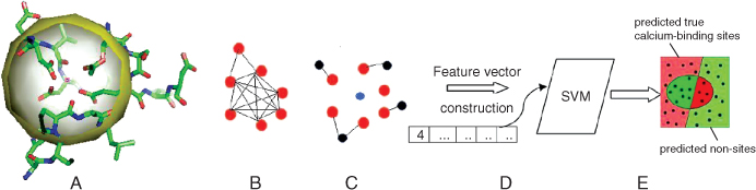
There is a significant meaning for the prediction performance to select an appropriate data encoding scheme to represent the microenvironments of calcium binding sites and nonsites because it largely determines the quality of feature extraction of SVM models. The spatial distributions of biophysical and biochemical properties surrounding calcium binding sites differ significantly from those surrounding the control nonsites [11]. For every putative calcium binding site, GSVM extract biophysical and biochemical properties from every spherical region into a feature vector. The feature descriptors of protein structure include four groups, atom-based features, chemical group–based features, residue-based features, and secondary structure–based features. The atom-based features consist of the number of carbons, number of nitrogens, number of oxygen atoms, sum of hydrophobicity values of all atoms within a putative calcium binding site, and sum of charge values of all atoms within a putative calcium binding site. Examples of chemical group–based feature include number of hydroxyls, number of amides, number of amines, number of carbonyls, number of ring structures, and number of peptides. Standard 20 amino acids can be classified into five groups: hydrophobic, charged, nonplolar, polar, and acidic. GSVM counted the number of amino acids within a putative calcium binding site for every group, then encoded into residue-based features. Secondary structure–based features include the number of ALPHA, the number of BETA, the number of COIL, and the number of HET within a putative calcium binding site. In one word, the spatial distributions of biophysical and biochemical properties for every (sphere, PCC) pair were encoded into a 20-dimensional feature vector. Figure 3.3c,d describes the construction of a feature vector.
Figure 3.3 Schematic diagram of GSVM: (a) 7.0-Å spherical region around a calcium ion; (b) the extracted oxygen atom (red dots) and constructed graph ![]() . (c) a maximal clique of size 6 in graph
. (c) a maximal clique of size 6 in graph ![]() with calcium center (blue dot) (the black dots represent carbon atoms located within the spherical region); (d) for the spherical region, construction of a feature vector (e.g., one feature is the number of atoms); (e) the feature vector is taken as the input variable for SVM that distinguishes sphere samples between calcium binding sites and non-calcium-binding sites.
with calcium center (blue dot) (the black dots represent carbon atoms located within the spherical region); (d) for the spherical region, construction of a feature vector (e.g., one feature is the number of atoms); (e) the feature vector is taken as the input variable for SVM that distinguishes sphere samples between calcium binding sites and non-calcium-binding sites.
3.2.5.4 Data Preprocessing
There are several hundreds of putative calcium binding sites found for every protein structure. The putative site is labeled as ![]() if the PCC of a putative site is located within 3.5 Å of the documented calcium ion; otherwise it is labeled
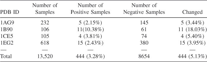
if the PCC of a putative site is located within 3.5 Å of the documented calcium ion; otherwise it is labeled ![]() . Unfortunately, the class imbalance problem exists because the number of positive site samples is relatively rare as compared with that of negative site samples. For example, given 1AG9, there are 5 positive samples but 232 negative samples. Since only support vectors (SVs) are used for classification and many majority samples far from the decision boundary can be removed without affecting the classification [21], SVM is more accurate on moderately imbalanced data compared with other standard classifiers. However, a SVM classifier can be sensitive to high class imbalance data, which results in a drop in the classification performance on the positive class. It is prone to generating a classifier that has a strong estimation bias toward the majority class, resulting in a large number of false negatives. The methods proposed to solve imbalanced classification can be categorized into the following three different types: cost-sensitive learning, oversampling the minority class, or undersampling the majority class [21].
. Unfortunately, the class imbalance problem exists because the number of positive site samples is relatively rare as compared with that of negative site samples. For example, given 1AG9, there are 5 positive samples but 232 negative samples. Since only support vectors (SVs) are used for classification and many majority samples far from the decision boundary can be removed without affecting the classification [21], SVM is more accurate on moderately imbalanced data compared with other standard classifiers. However, a SVM classifier can be sensitive to high class imbalance data, which results in a drop in the classification performance on the positive class. It is prone to generating a classifier that has a strong estimation bias toward the majority class, resulting in a large number of false negatives. The methods proposed to solve imbalanced classification can be categorized into the following three different types: cost-sensitive learning, oversampling the minority class, or undersampling the majority class [21].
There are 13,520 samples in dataset I where the positive:negative ratio is about 1:29 as shown in Table 3.2. If the PCC of a negative sample site falls within the cutoff distance (3.0 Å in our study) of its neighboring negative sample site, one of these two will be removed from the dataset. Thus, by removal of close negative spherical regions, majority negative samples are undersampled. The positive:negative ratio is reduced to 1:18 as shown in column, of Table 3.2; however, it is still highly imbalanced. The libsvm23 program implemented in RapidMiner [22] for binary classification was used with fivefold cross-validation. The cost matrix used for cost-sensitive learning was defined as [![]() ; 10 0], which means that the costs for the error of predicting
; 10 0], which means that the costs for the error of predicting ![]() as
as ![]() are 10 times higher than the other error type. The problem of imbalanced data is further alleviated through cost-sensitive learning.
are 10 times higher than the other error type. The problem of imbalanced data is further alleviated through cost-sensitive learning.
Table 3.2 Example of Imbalanced Data in Dataset II
3.3 Results and Discussion
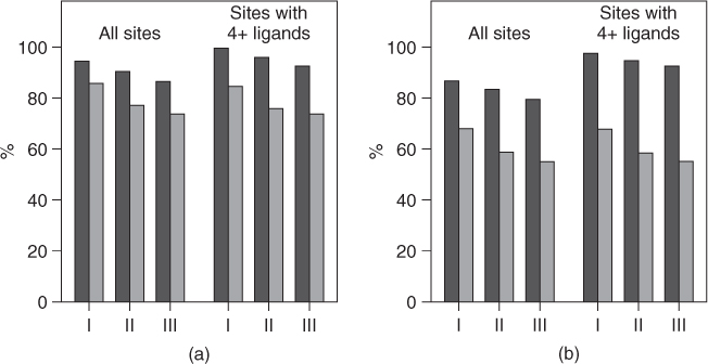
A SEN of 91% and a SEL of 77% have been achieved for the prediction of 91 calcium binding sites in dataset II when a true prediction is assumed if the predicted calcium is within 3.5 Å of the documented calcium ions by using an O![]() O cutoff of 6.0 Å a psdCa
O cutoff of 6.0 Å a psdCa![]() O range of 1.8–3.0 Å and a D-filter equal to psdCa
O range of 1.8–3.0 Å and a D-filter equal to psdCa![]() O. Under the same condition, a SEN of 87% and a SEL of 74% have been achieved in dataset III as shown in Figure 3.4a. The SEN and SEL are 84% and 59% for dataset II and 80% and 55% for dataset III, respectively (Fig. 3.4b) if the standard of a true prediction is that the predicted calcium is within 1 Å of the documented calcium ions. As in dataset I, 6 of 11 sites with three or fewer ligands in dataset II and 4 of 13 in dataset III have been identified within 3.5 Å of the real calcium, but none of the predictions is within 1 Å of the real calcium. If we consider only the calcium binding sites with four or more ligands as real sites, the SENs for datasets I, II, and III increase to 98%, 95%, and 93%, respectively, with the true prediction standard of within 1.0 Å of the documented calcium ions (as shown in Fig 3.4). Although the performance of the prediction was lower by including these less popular calcium binding sites or non-calcium-binding proteins, it confirms the practicability of high site selectivity, sensitivity, and accuracy of GG algorithm.
O. Under the same condition, a SEN of 87% and a SEL of 74% have been achieved in dataset III as shown in Figure 3.4a. The SEN and SEL are 84% and 59% for dataset II and 80% and 55% for dataset III, respectively (Fig. 3.4b) if the standard of a true prediction is that the predicted calcium is within 1 Å of the documented calcium ions. As in dataset I, 6 of 11 sites with three or fewer ligands in dataset II and 4 of 13 in dataset III have been identified within 3.5 Å of the real calcium, but none of the predictions is within 1 Å of the real calcium. If we consider only the calcium binding sites with four or more ligands as real sites, the SENs for datasets I, II, and III increase to 98%, 95%, and 93%, respectively, with the true prediction standard of within 1.0 Å of the documented calcium ions (as shown in Fig 3.4). Although the performance of the prediction was lower by including these less popular calcium binding sites or non-calcium-binding proteins, it confirms the practicability of high site selectivity, sensitivity, and accuracy of GG algorithm.
Figure 3.4 The sensitivity (black bars) and selectivity (gray bars) of the GG program with a O![]() O distance cutoff of 6.0 Å and the psdCa
O distance cutoff of 6.0 Å and the psdCa![]() O distance range cutoff of 1.8–3.0 Å. The standard of a true prediction is that the predicted calcium position is within 3.5 Å (a) or 1.0 Å (b) threshold distance to the documented calcium ions. The results of all sites are shown on the left, and the results considering only the sites with four or more ligands are shown on the right.
O distance range cutoff of 1.8–3.0 Å. The standard of a true prediction is that the predicted calcium position is within 3.5 Å (a) or 1.0 Å (b) threshold distance to the documented calcium ions. The results of all sites are shown on the left, and the results considering only the sites with four or more ligands are shown on the right.
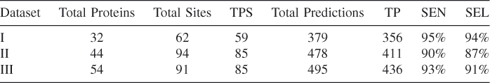
GSVM classified all (sphere, PCC) pairs into two types: calcium binding sites and non-calcium-binding sites. To obtain maximum accuracy, 20 experiments with fivefold cross-validation were conducted for every dataset. The summary results of experiments are presented in Table 3.3. For dataset I, the total predictions made by GSVM was 379 (column 5 in Table 3.3) and the total number of TPs was 356 (column 6 in Table 3.3), while 59 of 62 documented sites were predicted. Thus, the sensitivity was ![]() (column 7 in Table 3.3), whereas the selectivity was
(column 7 in Table 3.3), whereas the selectivity was ![]() (column 8 in Table 3.3).
(column 8 in Table 3.3).
Table 3.3 Summary Performance of Datasets I, II, and III
GG2.0 queried from the metalloprotein database and browser (MDB) [23] with the conditions that every calcium-binding protein structure from PDB [24] have a resolution ![]() Å from X-ray crystallography, each site have a coordination number
Å from X-ray crystallography, each site have a coordination number ![]() excluding water oxygen, and the PDB entry be in the PDBSELECT nonhomology list (Hobohm and Sander) in order to acquire a high-resolution and nonhomology dataset of proteins with calcium binding sites. The retrieved dataset contains 163 proteins of 345 sites. After excluding the PDB entries containing a calcium binding site that does not conform to the same requirement as the Fold-X method, we find that the training dataset contains 121 protein structure files with all 240 calcium binding sites finally. Four calcium binding sites a have coordinated ligand number of
excluding water oxygen, and the PDB entry be in the PDBSELECT nonhomology list (Hobohm and Sander) in order to acquire a high-resolution and nonhomology dataset of proteins with calcium binding sites. The retrieved dataset contains 163 proteins of 345 sites. After excluding the PDB entries containing a calcium binding site that does not conform to the same requirement as the Fold-X method, we find that the training dataset contains 121 protein structure files with all 240 calcium binding sites finally. Four calcium binding sites a have coordinated ligand number of ![]() each and are not taken into account for calculating prediction accuracy in the testing dataset containing 20 proteins.
each and are not taken into account for calculating prediction accuracy in the testing dataset containing 20 proteins.
As seen from Figure 3.5, without using the chemical filter, GG2.0 can obtain the prediction accuracy of the SENs ranging from 92% to 98% with SELs ranging from 87% to 78%. There is a tradeoff between the SEN and the corresponding SEL. Since SEN with a higher value than SEL is preferred, 74% is taken as the empirical value of ar_RO_RC for the filter threshold. Using the chemical filter with an ar_RO_RC of 75%, the GG2.0 obtains the best site sensitivity of 98%, but the SEL increases from 82% to 86%. This means that the chemical filter is the absolute filter to exclude non calcium-binding oxygen clusters.
Figure 3.5 Effect of ar_RO_RC on prediction accuracy.

Several methods such as Feature and SeqFeature based on the statistic function of the physicochemical environment around functional sites have been developed for predicting calcium-binding sites [5,6,7,8,9]. These methods predict the calcium binding sites by a scoring system taking into account multiple properties such as secondary structures, chemical groups, and atom types for which high sensitivity and selectivity have been claimed. The same dataset investigated by Altman et al. using Feature was analyzed by GG program [12]. The standard of true prediction of calcium binding sites is within 6.0 Å of the documented calcium for FEATURE in contrast to 1.0 Å for the prediction using GG. Even though the SEN from FEATURE is similar to that from the GG with the sacrifice of SEL for the sites with four or more oxygen ligand atoms, GG has achieved SEN of 95% within 1 Å of the structural resolution. The experimental results have shown that the GG program not only provided high prediction sensitivity without the use of vast statistical properties but also retained a greater site resolution to the documented calcium positions. This is very important for the application of testing the functions of the proteins with required resolution and accuracy. GG2.0 is an enhanced version of the GG method to predict calcium binding sites in proteins. it not only reduces the search space of the GG but also reveals certain geometric relation between the oxygen shell and carbon shell of calcium binding sites. Additionally, it indicates that some oxygen clusters from a group of residues with certain combination are formed possibly as a result of to hydrogen bonds instead of calcium ionic bonds. The two proposed filters in GG2.0 are useful for designing calcium binding sites in proteins. GSVM combines the advantages of GG and statistical methods. It is observed that GSVM has better site sensitivity and selectivity compared with GG. For two reasons: (1) the biophysical and biochemical properties of environments around sites are smoothly incorporated into feature vectors, so more features are used to select calcium binding sites; and (2) the SVM has superior generalization capability, and is a good tool for the binary classification problem. Moreover, GSVM actually builds a general model, which can be used to test numerous various features to identify significant ones related to forming calcium binding sites.
3.4 Conclusion
Identifying calcium binding sites is very important for the study of proteins. It is strongly needed to develop methodology for predicting calcium binding sites in proteins with high accuracy and high speed. Three methodologies are reviewed in this chapter, which are GG 17, GG2.0 20, and GSVM 21. GG using graph theory has revealed new features of calcium binding in proteins and the developed program may facilitate the understanding and prediction of functions of calcium roles in biological systems based on oxygen coordination, which can be provided by homology modeling based on the sequence information. GG can be a powerful tool for automated analysis of large structural genomic databases with sensitivity of ![]() in addition to its capability of provided structural resolution (within 1 Å of the documented ions and with high speed). The GG2.0, as an enhanced version of the GG method, reduces the search space of GG, and further captures certain geometric relation between the oxygen shell and the carbon shell of calcium binding sites. GSVM adopts a statistical learning method to classify calcium binding sites and nosites based on constructed regions using a graph algorithm. Thus, GSVM absorbs advantages of both statistical learning and graph theory. Moreover, GSVM provides a means for building a general model that can be used to test and select significant features directly related to forming calcium binding sites.
in addition to its capability of provided structural resolution (within 1 Å of the documented ions and with high speed). The GG2.0, as an enhanced version of the GG method, reduces the search space of GG, and further captures certain geometric relation between the oxygen shell and the carbon shell of calcium binding sites. GSVM adopts a statistical learning method to classify calcium binding sites and nosites based on constructed regions using a graph algorithm. Thus, GSVM absorbs advantages of both statistical learning and graph theory. Moreover, GSVM provides a means for building a general model that can be used to test and select significant features directly related to forming calcium binding sites.
References
1. Silva JJRF, Williams RJP, The Biological Chemistry of the Elements, Oxford Univ. Press, 1991.
2. Linse S, Forsen S, Determinants that govern high-affinity calcium binding, Adv. 2nd Messenger Phosphoprot. Res. 30:89–151 (1995).
3. Ikura M, Calcium binding and conformational response in ef-hand proteins, Trends Biochem. Sci. 21(1): 14–17 (1996).
4. Yang W, Lee HW, Hellinga H, Yang JJ, Structure analysis, identification and design of calcium-binding sites in proteins, Proteins 47:344–356 (2002).
5. Pidcock E, Moore GR, Structural characteristics of protein binding sites for calcium and lanthanide ions, J. Biol. Inorg. Chem. 6:479–489 (2001).
6. Yamashita MM, Wesson L, Eisenman G, Eisenberg D, Where metal ions bind in proteins, Proc. Natl. Acad. Sci. USA 87:5648–5652 (1990).
7. Nayal M, Di Cera E, Predicting Ca![]() -binding sites in proteins, Proc. Natl. Acad. Sci. USA 91:817–821 (1994).
-binding sites in proteins, Proc. Natl. Acad. Sci. USA 91:817–821 (1994).
8. Wei L, Huang ES, Altman RB, Are predicted structures good enough to preserve functional sites? Struct. Fold. Design 7:643–650 (1997).
9. Sodhi JS, Bryson K, McGuffin LJ, Ward JJ, Wernisch L, Jones DT, Predicting metal-binding site residues in low-resolution structural models, J. Mol. Biol. 342:307–332 (2004).
10. Kuntz ID, Blaney JM, Oatley SJ, Langridge R, Ferrin TE, A geometric approach to macromolecule-ligand interactions, J. Mol. Biol. 161:269–288 (1982).
11. Bagley SC, Altman RB, Characterizing the microenvironment surrounding protein sites. Protein Sci. 4:622–635 (1995).
12. Liang MP, Banatao DR, Klein TE, Brutlag DL, Altman RB, webFEATURE: An interactive web tool for identifying and visualizing functional sites on macromolecular structures, Nucleic Acids Res. 31:3324–3327 (2003).
13. Liang MP, Brutlag DL, Altman RB, Automated construction of structual motifs for predicting functional sites on protein structures, Proc. Pacific Symp. Biocomputing, pp. 2003, 204–215.
14. Katchalski-Katzir E, Shariv I, Eisenstein M, Friesem AA, Aflalo C, Vakser IA, Molecular surface recognition: determination of geometric fit between proteins and their ligands by correlation techniques, Proc. Natl. Acad. Sci. USA 89:2195–2199 (1992).
15. Rychlewski L, Fischer D, Elofsson A, LiveBench-6: Large-scale automated evaluation of protein structure prediction servers, Proteins 53(Suppl. 6): 542–547 (2003).
16. Deng H, Chen G, Yang W, Yang JJ, Predicting calcium-binding sites in proteins— a graph theory and geometry approach, Proteins 64:34–42 (2006).
17. Samudrala R, Moult J, A graph-theoretic algorithm for comparative modeling of protein structure, J. Mol. Biol. 279:287–302 (1998).
18. Canutescu AA, Shelenkov AA, Dunbrack RL Jr, A graph-theory algorithm for rapid protein side-chain prediction, Protein Sci. 12:2001–2014 (2003).
19. Liu H, Deng H, Identifying calcium-binding sites with oxygen-carbon shell geometric and chemic criteria: A graph-based approach, Proc. 2008 IEEE Int. Conf. Bioinform. Biomedi. (BIBM 2008), Philadelphia, PA, pp. 2008, 407–410.
20. Liu H, Metts N, Identifying calcium-binding sites in proteins by analyzing the microenvironment surrouding protein sites via SVMs, Proc. 2009 World Congress in Computer Science, Computer Engineering, and Applied Computing, Las Vegas, Nevada, pp. 834–839, 2009.
21. Akbani R, Kwek S, Japkowicz N, Applying support vector machines to imbalanced data sets, Proc. 15th Eur. Conf. Machine Learning, Pisa, Italy, pp. 39–50, 2004.
22. See http://rapid-i.com/.
23. Castagnetto J, Hennessy S, Roberts V, Getzoff E, Tainer J, Pique M, MDB: The metalloprotein database and browser at the scripps research institute, Nucleic Acids Res, 30(1): 379–382 (2002).
24. Berman HM, Westbrook J, Feng Z, Gilliland G, Bhat TN, Weissig H, Shindyalov IN, Bourne PE, The protein data bank, Nucleic Acids Res. 28(1): 235–242 (2000).