Chapter 14
Discovering 3D Protein Structures for Optimal Structure Alignment
TOMá![]() NOVOSáD, VáCLAV SNá
NOVOSáD, VáCLAV SNá![]() EL, AJITH ABRAHAM, and JACK Y. YANG
EL, AJITH ABRAHAM, and JACK Y. YANG
14.1 Introduction
Analyzing three-dimensional protein structures is a very important task in molecular biology. Nowadays, the solution for protein structures often stems from the use of the state-of-the-art technologies such as nuclear magnetic resonance (NMR) spectroscopy techniques or X-ray crystallography as seen in the increasing number of PDB [34] entries. The Protein Data Bank (PDB) is a database of 3D structural data of large biological molecules, such as proteins and nucleic acids. It was proved that structurally similar proteins tend to have similar functions even if their amino acid sequences are not similar to one another. Thus, it is very important to find proteins with similar structures (even in part) from the growing database to analyze protein functions. Yang et al. [47] exploited machine learning techniques, including variants of self-organizing global ranking, a decision tree, and support vector machine (SVM) algorithms to predict the tertiary structure of transmembrane proteins. Hecker et al. [14] developed a state-of-the-art protein disorder predictor and tested it on a large protein disorder dataset created from the PDB. The relationship between of sensitivity and specificity is also evaluated. Habib et al. [11] presented a new SVM-based approach to predict the subcellular locations based on amino acid and amino acid pair composition. More protein features can be factored in to improve the accuracy significantly. Wang et al. [45] discussed an empirical approach to specify the localization of protein binding regions utilizing information including the distribution pattern of the detected RNA fragments and the sequence specificity of RNase digestion. Another important aproach of protein structural similarity is based on database indexing methods. Gao and Zaki [9] proposed a method for indexing protein tertiary structure by extracting a protein local feature vectors and suffix trees. Shibuya [43] developed a structure called geometric suffix tree, which indexes protein 3D structures based on their C![]() atoms' 3D coordinates.
atoms' 3D coordinates.
These studies are often targeted mainly at some kind of selection of the PDB database. In our past work [28, 29] we focused on the task of computing all-to-all protein similarities, which appear in thecurrent PDB database, based on their 3D structural features. The structural similarity defined between any two proteins in PDB can be calculated using information retrieval methods and schemes and suffix trees. These methods were previously widely studied and are commonly used these days [5, 13, 21, 23, 49]. To be able to evaluate the precision of the methods used to determine the protein structural similarity, it is important to compare the results toward the existing state-of-the-art techniques or databases. The existing state-of-the-art databases of protein structural similarities include DALI [15], SCOP [42], and CATH [3].
14.2 Protein Structure
Proteins are large molecules that provide structure and control reactions in all cells. In many cases only a small part of the structure—an active site—is directly functional, and the remainder exists only to create and fix the spatial relationship among the active site residues [19]. Chemically, protein molecules are long polymers typically containing several thousand atoms, composed of a uniform repetitive backbone (or mainchain) with a particular sidechain attached to each residue. The amino acid sequence of a protein records the succession of sidechains. There are 20 different amino acids that make up essentially all protein molecules on Earth. Every amino acid has its own original design composed of a central carbon (also called the alpha carbon, C![]() ), which is bonded to hydrogen, carboxylic acid group, amino group and unique sidechain or R group (e.g., see Fig. 14.1). The chemical properties of the R group are what give an amino acid its character.
), which is bonded to hydrogen, carboxylic acid group, amino group and unique sidechain or R group (e.g., see Fig. 14.1). The chemical properties of the R group are what give an amino acid its character.
The Danish protein chemist K. U. Linderstrøm-Lang described the protein structure in three different levels: primary structure, secondary structure, and tertiary structure. For proteins composed of more than one subunit, J. D. Bernall called the assembly of the monomers the quaternary structure.
Figure 14.1 Chemical structure of two amino acids: (a) glycine; (b) alanine.
14.2.1 Primary Structure
The unique sequence of amino acids in a protein is termed the primary structure. When amino acids form a protein chain, a unique bond, termed the peptide bond, exists between two amino acids. The sequence of a protein begins with the amino of the first amino acid and continues to the carboxyl end of the last amino acid. Each amino acid has its own unique one-letter abbreviation (e.g., alanine—A, methionine—M, arginine—R). Thus the primary structure of the protein can be expressed as a string of these letters. Examples of protein primary structure encoding are as follows:
MVLSEGEWQLVLHVWAKVEADVAGHGQDILIRLFKSHPETLEKFDRVKHL...
MNIFEMLRIDEGLRLKIYKDTEGYYTIGIGHLLTKSPSLNAAKSELDKAI...
AYIAKQRQISFVKSHFSRQLEERLGLIEVQAPILSRVGDGTQDNLSGAEK...
14.2.2 Secondary Structure
The second level in the hierarchy of protein structure consists of the various spatial arrangements resulting from the folding of localized parts of a polypeptide chain; these arrangements are referred to as secondary structures [20]. These foldings are either in a helical shape, called the alpha helix (![]() helix) (which was first proposed by Linus Pauling et. al in 1951 [32]), or a beta-pleated sheet (
helix) (which was first proposed by Linus Pauling et. al in 1951 [32]), or a beta-pleated sheet (![]() sheet) shaped similar to the zigzag foldings of an accordion. The turns of the
sheet) shaped similar to the zigzag foldings of an accordion. The turns of the ![]() helix are stabilized by hydrogen bonding between every fourth amino acid in the chain. The
helix are stabilized by hydrogen bonding between every fourth amino acid in the chain. The ![]() -pleated sheet is formed by folding successive planes [35]. Each plane is five to eight amino acids long. Both
-pleated sheet is formed by folding successive planes [35]. Each plane is five to eight amino acids long. Both ![]() helices and
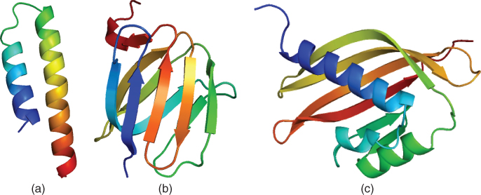
helices and ![]() sheets are linked by less structured loop regions to form domains (Fig. 14.2). The domains can potentionaly form fully functional proteins.
sheets are linked by less structured loop regions to form domains (Fig. 14.2). The domains can potentionaly form fully functional proteins.
Figure 14.2 Secondary structure elements and domain example: (a) ![]() helix; (b)
helix; (b) ![]() sheet; (c) domain.
sheet; (c) domain.
14.2.3 Tertiary Structure
The term tertiary structure (Fig. 14.3) refers to the overall conformation of a polypeptide chain, that is, the 3D arrangement of all its amino acid residues. Each atom of amino acid residue has its own 3D ![]() coordinates. In contrast with secondary structures, which are stabilized by hydrogen bonds, tertiary structure is stabilized primarily by hydrophobic interactions between the nonpolar sidechains, hydrogen bonds between polar sidechains, and peptide bonds. These stabilizing forces hold elements of secondary structure
coordinates. In contrast with secondary structures, which are stabilized by hydrogen bonds, tertiary structure is stabilized primarily by hydrophobic interactions between the nonpolar sidechains, hydrogen bonds between polar sidechains, and peptide bonds. These stabilizing forces hold elements of secondary structure ![]() helices,
helices, ![]() strands, turns, and random coils compactly together. The most the protein structures (∼90%) available in the Protein Data Bank have been resolved by X-ray crystallography. This method allows one to measure the 3D density distribution of electrons in the protein (in the crystallized state) and thereby infer the 3D coordinates of all the atoms to be determined to a certain resolution. Only ∼9% of the known protein structures have been obtained by nuclear magnetic resonance techniques (NMR spectroscopy) [2].
strands, turns, and random coils compactly together. The most the protein structures (∼90%) available in the Protein Data Bank have been resolved by X-ray crystallography. This method allows one to measure the 3D density distribution of electrons in the protein (in the crystallized state) and thereby infer the 3D coordinates of all the atoms to be determined to a certain resolution. Only ∼9% of the known protein structures have been obtained by nuclear magnetic resonance techniques (NMR spectroscopy) [2].
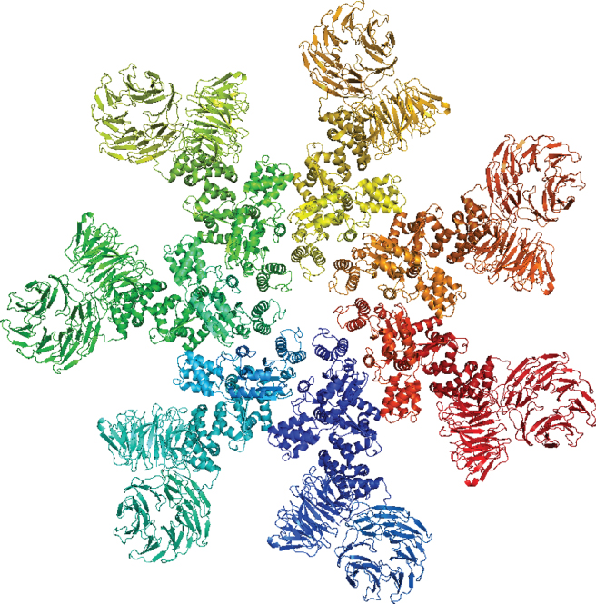
Figure 14.3 Tertiary structure of an apoptosome–procaspase 9 CARD complex.
14.2.4 Quaternary Structure
Some proteins need to functionally associate with others as subunits in a multimeric structure. This is called the quaternary structure of the protein. This can also be stabilized by disulfide bonds and by noncovalent interactions with reacting substrates or cofactors. An excellent example of quaternary structure is hemoglobin. Adult hemoglobin consists of two alpha (![]() ) subunits and two beta (
) subunits and two beta (![]() ) subunits, held together by noncovalent interactions [35].
) subunits, held together by noncovalent interactions [35].
14.3 Protein Databases
Currently there exist several protein databases publicly available online. These databases assembles various data about proteins, protein structures, protein functions, protein relationships, and other information. Probably the main and most valuable database is the PDB, which consists of protein 3D structures resolved by state-of-the-art techniques such as X-ray crystallography or NMR spectroscopy. Other online databases are generated by automated computer methods or by biologists themselves.
14.3.1 Protein Data Bank (PDB)
The PDB was established in 1971 at Brookhaven National Laboratory and originally contained seven structures. Nowadays the PDB archive contains almost 80,000 resolved structures and is still growing practically every day. The PDB archive is the single worldwide repository that contains information about experimentally determined structures of proteins, nucleic acids, and complex assemblies. The structures in the archive range from tiny proteins and bits of DNA to complex molecular machines like the ribosome. The structures in this archive is resolved by the state-of-the-art methods X-ray crystallography and NMR spectroscopy. As a member of the wwwPDB, the RCSB PDB curates and annotates PDB data according to established standards [34]. The PDB archive freely available to everyone and is updated each week at target time of Wednesday 00:00 UTC (Coordinated Universal Time). This database can be accessed online at http://www.pdb.org. The structures can also be downloaded from their FTP service at ftp://ftp.wwpdb.org/pub/pdb/.
14.3.2 Structural Classification of Proteins (SCOP)
This database provides a detailed and comprehensive description of the structural and evolutionary relationships of proteins whose 3D structures have been determined by X-ray crystallography or NMR spectroscopy (PDB entries). The most recent version 1.75 (June 2009) of this database includes 38,221 PDB entries. Classification of protein structures in the database is based on evolutionary relationships and on the principles that govern their 3D structure. The method used to construct the protein classification in SCOP is essentially the visual inspection and comparison of structures, although various automatic tools are used to make the task manageable and help provide generality [24–27, 42]. Each protein entry in the SCOP database (each chain of protein, respectively) is classified into the class, folding pattern, superfamily, family, domain, and species categories. These categories are hierarchically arranged from class to species. The SCOP database is accessible at no cost for the user at http://scop.mrc-lmb.cam.ac.uk/scop/.
14.3.3 CATH Protein Structure Classification
The CATH is a database constructed using a semiautomatic method for hierarchical classification of protein domains [31]. The CATH stands for class, architecture, topology and homologous superfamily. CATH shares many broad features with its main rival, SCOP; however there are also many areas in which the detailed classification differs greatly. CATH defines four classes: mostly ![]() , mostly
, mostly ![]() ,
, ![]() and
and ![]() and a few secondary structures. Much of the work in the CATH database is done by automatic methods toward the SCOP, although there are important manual tasks in the classification. The most important step in CATH classification is to separate the proteins into domains. The domains are next automatically sorted into classes and clustered on the basis of sequence similarities. These clusters (groups) form the H levels of the classification (homologous superfamily groups). The topology level is formed by structural comparisons of the homologous groups. Finally, the architecture level is assigned manually [31]. For more detailed descriptions of the CATH database building process and comparison with SCOP and other databases, please see References 6 and 12. The CATH database can be accessed and searched at http://www.cathdb.info/.
and a few secondary structures. Much of the work in the CATH database is done by automatic methods toward the SCOP, although there are important manual tasks in the classification. The most important step in CATH classification is to separate the proteins into domains. The domains are next automatically sorted into classes and clustered on the basis of sequence similarities. These clusters (groups) form the H levels of the classification (homologous superfamily groups). The topology level is formed by structural comparisons of the homologous groups. Finally, the architecture level is assigned manually [31]. For more detailed descriptions of the CATH database building process and comparison with SCOP and other databases, please see References 6 and 12. The CATH database can be accessed and searched at http://www.cathdb.info/.
14.3.4 Distance Matrix Alignment (DALI)
The DALI database is based on exhaustive all-against-all 3D structure comparison of protein structures currently in the PDB. The structural neighborhoods and alignments are automatically maintained and regularly updated using the DALI search engine. The DALI algorithm works with 3D coordinates of each protein that are used to calculate residue-to-residue (C![]()
![]() C
C![]() ) distance matrices. The distance matrices are first decomposed into elementary contact patterns, such ashexapeptide–hexapeptide submatrices. Then, similar contact patterns in the two matrices are paired and combined into larger consistent sets of pairs. This method is fully automatic and identifies structural resemblances and common structural cores accurately and sensitively, even in the presence of geometric distortions [15, 16]. The DALI database can be accessed from the DALI server at http://ekhidna.biocenter.helsinki.fi/dali.
) distance matrices. The distance matrices are first decomposed into elementary contact patterns, such ashexapeptide–hexapeptide submatrices. Then, similar contact patterns in the two matrices are paired and combined into larger consistent sets of pairs. This method is fully automatic and identifies structural resemblances and common structural cores accurately and sensitively, even in the presence of geometric distortions [15, 16]. The DALI database can be accessed from the DALI server at http://ekhidna.biocenter.helsinki.fi/dali.
14.4 Vector Space Model
The vector model [1] of documents was established in the 1970s [37, 38]. A document in the vector model is represented as a vector. Each dimension (element) of this vector corresponds to a separate term appearing in document collection. If a term occurs in the document, its value in the vector is nonzero. The vector model is a widely used information retrieval scheme for measuring similarity between documents or between user query and documents in the collection [7, 17, 18, 23, 28, 29, 39, 41].
In the vector model there are ![]() different terms
different terms ![]() for indexing
for indexing ![]() documents. Then each document
documents. Then each document ![]() is represented by a vector
is represented by a vector
![]()
where ![]() is the weight of the term
is the weight of the term ![]() in the document
in the document ![]() . These term weights is ultimately used to compute the degree of similarity between all documents stored in the system and the user query. The weight of the term in the document vector can be determined in many ways. A common approach uses the so-called (term frequency
. These term weights is ultimately used to compute the degree of similarity between all documents stored in the system and the user query. The weight of the term in the document vector can be determined in many ways. A common approach uses the so-called (term frequency ![]() inverse document frequency (TF
inverse document frequency (TF ![]() IDF)) method [40], in which the weight of the term is determined by the frequency with which the term
IDF)) method [40], in which the weight of the term is determined by the frequency with which the term![]() occurs in the document
occurs in the document ![]() (the term frequency TF
(the term frequency TF![]() ) and how often it occurs in the whole document collection (the document frequency DF
) and how often it occurs in the whole document collection (the document frequency DF![]() ). Precisely, the weight of the term
). Precisely, the weight of the term ![]() in the document
in the document ![]() is [8]
is [8]
where IDF stands for the inverse document frequency. This method assigns high weights to terms that appear frequently in a small number of documents in the document set.
An index file of the vector model is represented by the matrix
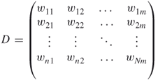
where the ![]() th row matches the
th row matches the ![]() th document and the
th document and the ![]() th column matches the
th column matches the ![]() th term.
th term.
The similarity between two documents in the vector model is usually expressed by the following formula (termed the cosine similarity measure):
14.2 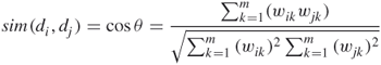
Suppose that we have two documents ![]() and
and ![]() , where
, where ![]() ,
, ![]() represent the weights of terms
represent the weights of terms ![]() ;
; ![]() , in document
, in document ![]() ; and
; and ![]() ,
, ![]() , the weights of terms
, the weights of terms ![]() ,
, ![]() in document
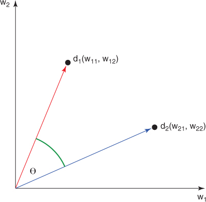
in document ![]() . Then the geometric representation of cosine similarity is as shown in Figure 14.4.
. Then the geometric representation of cosine similarity is as shown in Figure 14.4.
Figure 14.4 Geometric representation of cosine similarity.
For more information about the vector space model, please consult the literature [1, 22, 33, 37–39].
14.5 Suffix Trees
A suffix tree is a data structure that allows efficient string matching and querying. Suffix trees have been studied and used extensively, and have been applied to fundamental string problems such as finding the longest repeated substring [46], string comparisons [8], and text compression [36]. Following this, we describe the suffix tree data structure—its definition, construction algorithms, and main characteristics.
14.5.1 Definitions
The following description of the suffix tree was taken from Gusfield's book Algorithms on Strings, Trees and Sequences [10]. Suffix trees commonly deal with strings as a sequence of characters. One major difference is that we treat documents as sequences of words, not characters. A suffix tree of a string is simply a compact trie (a trie is also termed a digital tree or a prefix tree) of all the suffixes of that string. Zamir [48] provides the following definition.
In cases where one suffix of ![]() matches a prefix of another suffix of
matches a prefix of another suffix of ![]() , then no suffix tree obeying Definition 14.1 is possible since the path for the first suffix would not end at a leaf. To avoid this, we assume that last word of
, then no suffix tree obeying Definition 14.1 is possible since the path for the first suffix would not end at a leaf. To avoid this, we assume that last word of ![]() does not appear anywhere else in the string. This prevents any suffix from being a prefix to another suffix. To achieve this, we can add a terminating character, which is not in the language that
does not appear anywhere else in the string. This prevents any suffix from being a prefix to another suffix. To achieve this, we can add a terminating character, which is not in the language that ![]() is taken from, to the end of
is taken from, to the end of ![]() .
.
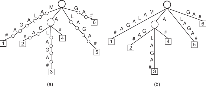
Suppose that we have a short protein sequence MALAGA that is a combination of four amino acids: methionine, alanine, leucine and glycine. An example of a suffix trie of the string MALAGA# is shown in Figure 14.5a. A corresponding suffix tree of the string MALAGA# is presented in Figure 14.5b. There are six leaves in this example, marked as rectangles and numbered from 1 to 6. The terminating characters are also shown in this figure.
Figure 14.5 Simple example of suffix trie and suffix tree of string MALAGA#: (a) suffix trie; (b) suffix tree.
In a similar manner, a suffix tree of a set of strings, called a generalized suffix tree [10], is a compact trie of all the suffixes of all the strings in the set [48], defined as follows.
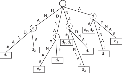
Figure 14.6 is an example of a generalized suffix tree of the set of two strings: RNADNA# and DNARNA#. The internal nodes of the suffix tree are drawn as circles, and are labeled from a to d. Leaves are drawn as rectangles, and numbers ![]() ) in each rectangle indicate the string from which that suffix originates—a unique number that identifies the string. Each string is considered to have a unique terminating symbol.
) in each rectangle indicate the string from which that suffix originates—a unique number that identifies the string. Each string is considered to have a unique terminating symbol.
Figure 14.6 Example of the generalized suffix tree.
14.5.2 Suffix Tree Construction Algorithms
The naive, straightforward method for building a suffix tree for a string ![]() of length
of length ![]() takes
takes ![]() time. The naive method first enters a single edge for the suffix
time. The naive method first enters a single edge for the suffix ![]() into the tree. Then it successively enters the suffix
into the tree. Then it successively enters the suffix ![]() into the growing tree for
into the growing tree for ![]() increasing from 2 to
increasing from 2 to ![]() . The details of this construction method are beyond the scope of this chapter. Various suffix tree construction algorithms can be found in Gusfield's text [10] (a good source on suffix tree construction algorithms in general).
. The details of this construction method are beyond the scope of this chapter. Various suffix tree construction algorithms can be found in Gusfield's text [10] (a good source on suffix tree construction algorithms in general).
Several linear time algorithms for constructing suffix trees exist [30, 44, 46]. To be precise, these algorithms also exhibit a time dependence on the size of the vocabulary (or the alphabet when dealing with character-based trees); they actually have a time bound of ![]() , where
, where ![]() is the length of the string and
is the length of the string and ![]() is the size of the language. These methods are more difficult to implement than the naive method, which is sufficiently suitable for our purpose.
is the size of the language. These methods are more difficult to implement than the naive method, which is sufficiently suitable for our purpose.
Some implementation improvements of the naive method can also be made to improve the ![]() worst-case time bound. With these improvements, it can achieve constant access time for finding an appropriate child of the root (this is important because the root node has the same count or number of child nodes as the number of letters in the alphabet—count of terms in document collection) and logarithmic time needed to find an existing child or to insert a new child node in any other internal nodes of the tree [10, 23].
worst-case time bound. With these improvements, it can achieve constant access time for finding an appropriate child of the root (this is important because the root node has the same count or number of child nodes as the number of letters in the alphabet—count of terms in document collection) and logarithmic time needed to find an existing child or to insert a new child node in any other internal nodes of the tree [10, 23].
14.6 Indexing 3D Protein Structures
As was mentioned above, the data for protein 3D structures indexing are retrieved from PDB database, which consists of proteins, nucleic acids, and complex assemblies. Before indexing protein structures, we consider only complete protein structures. We filter out all nucleic acids and complex assemblies from the entire PDB database. Next we filter out proteins, which have incomplete N![]() C
C![]()
![]() C
C![]() O backbones (e.g., some of the files have C atoms in the protein backbone missing). After this cleaning step, we have a collection of files containing a description of a specific protein and its 3D structure and containing only amino acid residues with complete a N
O backbones (e.g., some of the files have C atoms in the protein backbone missing). After this cleaning step, we have a collection of files containing a description of a specific protein and its 3D structure and containing only amino acid residues with complete a N![]() C
C![]()
![]() C
C![]() O atom sequence. Each retrieved file has at least one mainchain (some proteins have more than one mainchain) of at least one model (some PDB files contained more models of 3D protein structure). In cases when the PDB file contained multiple chains or models, we took into account all of those (all mainchains of all models).
O atom sequence. Each retrieved file has at least one mainchain (some proteins have more than one mainchain) of at least one model (some PDB files contained more models of 3D protein structure). In cases when the PDB file contained multiple chains or models, we took into account all of those (all mainchains of all models).
To be able to measure 3D protein structure similarity using suffix treesand the vector space model, we need to encode protein 3D structure into a vector representation. This can be achieved in various ways [4, 9, 16, 28, 50].
14.6.1 Torsion Angles
Any plane can be defined by two noncollinear vectors lying in that plane; taking their crossproduct and normalizing yields the normal unit vector to the plane. Thus, a torsion angle can be defined by four pairwise noncollinear vectors.
The backbone torsion angles of proteins are called ![]() (phi, involving the backbone atoms C
(phi, involving the backbone atoms C![]() N
N![]() C
C![]()
![]() C),
C), ![]() (psi, involving the backbone atoms N
(psi, involving the backbone atoms N![]() C
C![]()
![]() C
C![]() N) and
N) and ![]() (omega, involving the backbone atoms C
(omega, involving the backbone atoms C![]()
![]() C
C![]() N
N![]() C
C![]() ). Thus,
). Thus, ![]() controls the C
controls the C![]() C distance,
C distance, ![]() controls the N
controls the N![]() N distance and
N distance and ![]() controls the C
controls the C![]()
![]() C
C![]() distance.
distance.
The planarity of the peptide bond usually restricts ![]() to be 180
to be 180![]() (the typical trans case) or 0
(the typical trans case) or 0![]() (the rare cis case). The
(the rare cis case). The ![]() and
and ![]() torsion angles tend to range from
torsion angles tend to range from ![]() to 180
to 180![]() .
.
14.6.2 Encoding the 3D Protein Mainchain Structure for Indexing
To be able to index proteins by information retrieval (IR) techniques, we need to encode the 3D structure of the protein backbone into some sequence of characters, words, or integers (as in our case). The area of protein 3D structure encoding has been widely studied [e.g., [4, 9, 50]. Since the protein backbone is the sequence of the amino acid residues (in 3D space), we are able to encode this backbone into the sequence of integers in the following manner.
For example, let us say that the protein backbone consists of six amino acid residues RNADNA (abbreviations for arginine, asparagine, alanine, and aspartic acid). The relationship between the two following residues can be described by their torsion angles ![]() ,
, ![]() , and
, and ![]() . Since
. Since ![]() and
and ![]() take values from the interval
take values from the interval ![]() , this must be done with some normalization. From this interval we can obtain discrete values by dividing the interval into equal-sized subintervals (e.g., into 36 subintervals; e.g.,
, this must be done with some normalization. From this interval we can obtain discrete values by dividing the interval into equal-sized subintervals (e.g., into 36 subintervals; e.g., ![]() ,
, ![]() ,
, ![]() ). Each of these values was labeled with nonnegative integers as follows: 00, 01,…, 36 where 00 stands for
). Each of these values was labeled with nonnegative integers as follows: 00, 01,…, 36 where 00 stands for ![]() . Now, let's say that
. Now, let's say that ![]() is
is ![]() ; the closest discrete value is
; the closest discrete value is ![]() , which has the label 16, so we have encoded this torsion with the string 16. The same holds true for
, which has the label 16, so we have encoded this torsion with the string 16. The same holds true for ![]() . Torsion angle
. Torsion angle ![]() was encoded as either of the two characters A or B since the
was encoded as either of the two characters A or B since the ![]() tends to be almost in every case
tends to be almost in every case ![]() or
or ![]() . After concatenation of these three parts we obtain a string that looks something like A0102, which means that
. After concatenation of these three parts we obtain a string that looks something like A0102, which means that ![]() ,
, ![]() ,
, ![]() . Concatenation was done in the following manner:
. Concatenation was done in the following manner:![]() .
.
The suffix tree can index sequences of characters, numbers, words, and so on. To conserve computer memory space, it is better to represent the sequence of words with a sequence of nonnegative integers. For example, let's say that we have a protein with a backbone consisting of six residues, such as RNADNA with its 3D properties. The resulting encoded sequence can be, for example; {A3202, A2401, A2603, A2401, A2422, A2422, A2220}.
After obtaining this six-word sequence, we create a dictionary of these words (each unique word receives its own unique nonnegative integer identifier). The translated sequence appears as {0, 1, 2, 1, 3, 3, 4}.
In this way, we can encode each mainchain of each model contained into one PDB file. This task is done for every protein included in our filtered PDB collection. Now we are ready to index proteins using suffix trees.
14.7 Protein Similarity Algorithm
We describe the algorithm for measuring protein similarity on the basis of their tertiary structure [28, 29]. A brief description of the algorithm follows:
14.7.1 Inserting All Mainchains into the Suffix Tree
At this stage of the algorithm, we construct a generalized suffix tree of all encoded mainchains. As mentioned in Section 14.6, we obtain the encoded forms of 3D protein mainchains—sequences of positive numbers. All of these sequences are inserted into the generalized suffix tree data structure (Section 14.5).
14.7.2 Finding All Maximal Substructure Clusters
To build a vector model of proteins, we have to find all maximal phrase clusters. Recall the example given in Section 14.6, namely, that the phrases can be RNADNA#, RNA#, DNA#, and so on (just imagine that phrase RNA# is equal to A3202 A2401 A2603 #). The phrase in the present context is an encoded protein mainchain or any of its parts. The document in our context can be seen as a set of encoded mainchains of the protein. Now we can define a maximal phrase cluster (the longest common substructure; see Fig. 14.7) [49].
Figure 14.7 Example of maximal phrase cluster: nodes b and c.
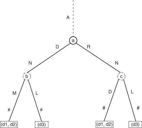
Now we simply traverse the generalized suffix tree and identify all maximal phrase clusters (i.e., all of the longest common substructures). A maximal phrase cluster can be seen as a kind of 3D structural alignment—common parts of 3D protein structure shared between two or more proteins. Figure 14.7 displays the example of maximal phrase cluster.
14.7.3 Building a 3D Protein Structure Vector Model
We describe the procedure for building the matrix representing the vector model index file (Section 14.4). In a classical vector space model, the document is represented by the terms (which are words), respectively, and by the weights of the terms. In our model the document is represented not by the terms but by the common phrases (maximal phrase clusters)! The term in our context is a common phrase, that is, a maximal phrase cluster.
In the previous stage of the algorithm, we identified all maximal phrase clusters—all the longest common substructures. From the definition of the phrase cluster, we know that the phrase cluster is the group of documents sharing the same phrase (group of proteins sharing the same substructure). Now we can obtain the matrix representing the vector model index file directly from the generalized suffix tree. Each document (protein) is represented by the maximal phrase clusters in which it is contained. For computing the weights of the phrase clusters, we are using a TF ![]() IDF weighting schema as given by Equation (14.1).
IDF weighting schema as given by Equation (14.1).
Let us say consider a simple example that we have a phrase cluster containing documents ![]() . These documents share the same phrase
. These documents share the same phrase ![]() . We compute
. We compute ![]() values for all documents appearing in a phrase cluster sharing the phrase
values for all documents appearing in a phrase cluster sharing the phrase ![]() . This task is done for all phrase clusters identified by the previous stage of the algorithm.
. This task is done for all phrase clusters identified by the previous stage of the algorithm.
Now we have a complete matrix representing the index file in a vector space model (see Section 14.4).
14.7.4 Building a Similarity Matrix
In the previous stage of the algorithm, we constructed a vector model index file. To build a protein similarity matrix, we use standard information retrieval techniques for measuring the similarity in a vector space model. As mentioned in Section 14.4, we have used cosine similarity, which appears to be quite suitable for our purpose. The similarity matrix is given by the following documents (proteins) similarity matrix:
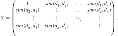
Here, the ![]() th row matches the
th row matches the ![]() th document (protein, respectively), and the
th document (protein, respectively), and the ![]() th column matches the
th column matches the ![]() th document (protein). The similarity matrix is diagonally symmetric.
th document (protein). The similarity matrix is diagonally symmetric.
14.7.5 Finding Similar Proteins
This step is quite simple. When we have computed the similarity matrix ![]() , we simply sort the documents (proteins) on each row according to their similarity scores. The higher the score, the more similar the two proteins are. We do this for each protein in our protein collection. The results of the algorithm can be found in [28].
, we simply sort the documents (proteins) on each row according to their similarity scores. The higher the score, the more similar the two proteins are. We do this for each protein in our protein collection. The results of the algorithm can be found in [28].
14.8 Summary
Analysis of 3D protein structures is an important part of current bioinformatics. It is a key part of discovering protein–protein interactions, necessitating efficient algorithms. Since the current protein databank (PDB) is growing almost every week and new structures have been discovered by NMR or X-ray crystallography very successfully, algorithms that can process large amounts of data are essential. Protein indexing algorithms can very efficiently discover the protein interactions on the basis of their tertiary structures and can be useful for building protein interactions networks, prediction of protein functions, fold recognition, homology detection, alignment of 3D protein structures, drug discovery, and other purposes.
References
1. Baeza-Yates R, Ribeiro-Neto B, Modern Information Retrieval, Adison-Wesley, 1999.
2. Bünger AT, X-PLOR, Version 3.1. A System for X-ray Crystallography and NMR, Yale Univ. Press, New Haven, CT, 1992.
3. CATH: Protein Structure Classification http://www.cathdb.info/; last accessed 7/10/09.
4. Chew LP, Huttenlocher D, Kedem K, Kleinberg J, Fast detection of common geometric substructure in proteins, J. Comput. Biol. 6(3/4):313–326 (1999).
5. Chim H, Deng X, A new suffix tree similarity measure for document clustering, Proc. 16th Int. Conf. World Wide Web (WWW 2007), ACM, New York, 2007, pp. 121–130.
6. Day R, Beck DA, Armen RS, Daggett V, A consensus view of fold space: Combining SCOP, CATH, and the Dali Domain Dictionary, Sci. 12(10):2150–2160 (2003).
7. Dráždilová P, Dvorský J, Martinovi![]() J, Snášel V, Search in documents based on topical development, in AWIC 2009, Amazon.ca, 2009.
J, Snášel V, Search in documents based on topical development, in AWIC 2009, Amazon.ca, 2009.
8. Ehrenfeucht A, Haussler D, A new distance metric on strings computable in linear time, Appl. Math. 20(3):191–203 (1988).
9. Gao F, Zaki MJ, PSIST: Indexing protein structures using suffix trees, Proc. IEEE Computational Systems Bioinformatics Conference (CSB), 2005, pp. 212–222.
10. Gusfield D, Algorithms on Strings, Trees and Sequences: Computer Science and Computational Biology, Cambridge Univ. Press, 1997.
11. Habib T, Zhang C, Yang JY, Yang MQ, Deng Y, Supervised learning method for the prediction of subcellular localization of proteins using amino acid and amino acid pair composition, BMC Genomics 9(Suppl. 1):S16 (2008).
12. Hadley C, Jones DT, A systematic comparison of protein structure classifications: SCOP, CATH and FSSP, Structure 7(9):1099–1112 (1999).
13. Hammouda KM, Kamel MS, Efficient phrase-based document indexing for web document clustering, IEEE Trans. Knowl. Data Eng. 16(10):1279–1296 (2004).
14. Hecker J, Yang JY, Cheng J, Protein disorder prediction at multiple levels of sensitivity and specificity, BMC Genomics 9(Suppl. 1):S9 (2008).
15. Holm L, Sander C, Dali: A network tool for protein structure comparison, Trends Biochem. Sci. 20(11):478–480 (1995).
16. Holm L, Sander C, Protein structure comparison by alignment of distance matrices, J. Mol. Biol. 233:123–138 (1993).
17. Hruška P, Martinovi![]() J, Dvorský J, Snášel V, XML Compression Improvements Based on the Clustering of Elements, CISIM, Poland, 2010.
J, Dvorský J, Snášel V, XML Compression Improvements Based on the Clustering of Elements, CISIM, Poland, 2010.
18. Lee DL, Chuang H, Seamons KE, Document ranking and the vector-space model, IEEE Software, 1997, pp. 67–75.
19. Lesk AM, Introduction to Bioinformatics, Oxford Univ. Press, 2008.
20. Lodish H, Berk A, Matsudaira P, Kaiser AC, Krieger M, Scott PM, Zipursky L, Darnell J, Molecular Cell Biology, 6th ed. Freeman WH, 2007.
21. Lexa M, Snášel V, Zelinka I, Data-mining protein structure by clustering, segmentation and evolutionary algorithms, in Data Mining: Theoretical Foundations and Applications, Springer-Verlag, Studies in Computational Intelligence Series, vol. 204, 2009, pp. 221–248.
22. Manning CD, Raghavan P, Schütze H, Introduction to Information Retrieval, Cambridge Univ. Press, 2008.
23. Martinovi![]() J, Novosád T, Snášel V, Vector Model Improvement Using Suffix Trees, IEEE, ICDIM, 2007, pp. 180–187.
J, Novosád T, Snášel V, Vector Model Improvement Using Suffix Trees, IEEE, ICDIM, 2007, pp. 180–187.
24. Murzin AG, Brenner SE, Hubbard T, Chothia C, SCOP: A structural classification of proteins database for the investigation of sequences and structures, J. Mol. Biol. 247:536–540 (1995).
25. Lo Conte L, Brenner SE, Hubbard TJP, Chothia C, Murzin A, SCOP database in 2002: Refinements accommodate structural genomics, Nucleic Acids Res. 30(1):264–267 (2002).
26. Andreeva A, Howorth D, Brenner SE, Hubbard TJP, Chothia C, Murzin AG, SCOP database in 2004: Refinements integrate structure and sequence family data, Nucleic Acids Res. 32:D226–D229 (2004).
27. Andreeva A, Howorth D, Chandonia J-M, Brenner SE, Hubbard TJP, Chothia C, Murzin AG, Data growth and its impact on the SCOP database: New developments. Nucleic Acids Res. 36:D419–D425 (2008).
28. Novosád T, Snášel V, Abraham A, Yang JY, Prosima—protein similarity algorithm, Proc. World Congress on Nature and Biologically Inspired Computing, 2009, pp. 84–91.
29. Novosád T, Snášel V, Abraham A, Yang JY, Searching protein 3-D structures for optimal structure alignment using intelligent algorithms and data structures, IEEE Trans. Inform. Technol. Biomed. 14(6):1378–1386 (2010).
30. McCreight E, A space-economical suffix tree construction algorithm, J. ACM 23:262–272 (1976).
31. Orengo CA, Michie AD, Jones S, Jones DT, Swindells MB, Thornton JM, CATH—a hierarchic classification of protein domain structures, Structure 5(8):1093–1108 (1997).
32. Pauling L, Corey RB, Branson HR, The structure of proteins; two hydrogen-bonded helical configurations of the polypeptide chain, Proc. Natl. Acad. Sci. USA 4:205–211 (1951).
33. van Rijsbergen CJ, Information Retrieval, 2nd ed., Butterworths, London, 1979.
34. RCSB Protein Databank—PDB (http://www.pdb.org)
35. Robinson R, Genetics, Macmillan Reference USA (2002).
36. Rodeh M, Pratt VR, Even S, Linear algorithm for data compression via string matching, J. ACM 28(1):16–24 (1981).
37. Salton G, The SMART Retrieval System—Experiments in Automatic Document Processing, Prentice-Hall, Englewood Cliffs, NJ, 1971.
38. Salton G, Lesk ME, Computer evaluation of indexing and text processing, J. ACM 15(1):8–36 (1968).
39. Salton G, Wong A, Yang CS, A vector space model for automatic indexing, Commun. ACM 18(11): (1975).
40. Salton G, Buckley C, Term-weighting approaches in automatic text retrieval, Inform. Process. Manage. 24(5):513–523 (1988).
41. Sarkar IN, A vector space model approach to identify genetically related diseases, J. Am. Med. Inform. Assoc. 19(2):249–254 (2012).
42. SCOP: A Structural Classification of Proteins Database for the Investigation of Sequences and Structure http://scop.mrc-lmb.cam.ac.uk/scop/; last accessed 7/10/09.
43. Shibuya T, Geometric suffix tree: A new index structure for protein 3D structures, in Combinatorial Pattern Matching, LNCS series, vol. 4009, 2006, pp. 84–93.
44. Ukkonen E, On-line construction of suffix trees, Algorithmica 14:249–260 (1995).
45. Wang Xin, Wang G, Shen C, Li L, Wang Xinguo, Mooney SD, Edenberg HJ, Sanford JR, Liu Y, Using RNase sequence specificity to refine the identification of RNA-protein binding regions, BMC Genomics 9(Suppl. 1):S17 (2008).
46. Weiner P, Linear pattern matching algorithms, Proc. 14th Annual Sympo. Foundations of Computer Science, 1973, pp. 1–11.
47. Yang JY, Yang MQ, Dunker AK, Deng Y, Huang X, Investigation of transmembrane proteins using a computational approach, BMC Genomics 9(Suppl. 1):S7 (2008).
48. Zamir O, Clustering Web Documents: A Phrase-Based Method for Grouping Search Engine Results, doctoral dissertation, Univ. Washington, 1999.
49. Zamir O, Etzioni O, Web document clustering: A feasibility demonstration, Proc. Special Interest Group on Information Retrieval Conf., (SIGIR'98), 1998, pp. 46–54.
50. Ye J, Janardan R, Liu S, Pairwise protein structure alignment based on an orientation-independent backbone representation, J. Bioinformatics Comput. Biol. 2:699–718 (2004).