
Chapter 13
Fundamentals of Protein Structure Alignment
13.1 Introduction
The central dogma of molecular biology asserts a one-way transfer of information from a cell's genetic code to the expression of proteins. Proteins are the functional workhorses of a cell, and studying these molecules is at the foundation of much of computational biology. Our goal here is to present a succinct introduction to the biological, mathematical, and computational aspects of making pairwise comparisons between protein structures. The presentation is intended to be useful for those who are entering this research area. The chapter begins with a brief introduction to the biology of protein comparison, which is followed by a brief taxonomy of the different mathematical frameworks for protein structure alignment. We conclude with a couple of more recent pairwise comparison techniques that are at the forefront of efficiency and accuracy. Such methods are becoming important as structural databases grow.
13.2 Biological Motivation of Protein Structure Alignment
Proteins are crucially important molecules that are responsible for a large variety of biological functions required for life to exist. The DNA sequence of the genome provides a one-dimensional descriptive code; proteins are self-organizing systems that allow expansion of this one-dimensional code into complex three-dimensional structures possessing a great diversity of functions. Understanding the types of protein structures that are possible is an important part of understanding the existing biological systems, of understanding the aberrant processes that result in genetic disorders, and in the engineering of proteins with novel functions.
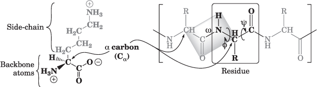
Proteins are synthesized as linear polymers of amino acids (Fig. 13.1); the vast majority of proteins consist of a set of 20 different types of amino acids, in defined sequences that, depending on the protein, vary from about 50 to more than 28,000 amino acid residues. Although there are exceptions, in general, the specific sequence of amino acids is specified by the genome; this linear sequence determines the 3D structure of the protein.
Figure 13.1 The structure of one type of amino acid (lysine) is shown on the left, with the sidechain and backbone atoms indicated. Proteins consist of amino acid residues, where the backbone atoms are linked together to form the chain, and the sidechains determine the folded structure and much of the function of the protein. In the partial protein shown on the right, the sidechains are denoted as R, and the three types of dihedral angles (the specific angle formed by the atoms bonded at each position along the backbone) are shown. The ![]() and
and ![]() angles may vary, within geometric limits imposed by the surrounding atoms; the
angles may vary, within geometric limits imposed by the surrounding atoms; the ![]() angle is fixed, with the six atoms forming the planar structure shown.
angle is fixed, with the six atoms forming the planar structure shown.
The 3D structure of a protein is an emergent property of the linear sequence. Predicting the 3D structure entirely on the basis of the linear sequence has proved to be challenging because the defined structure exhibited by most proteins is a consequence of a large number of relatively weak interactions. The existence of a defined structure is possible because of geometric constraints imposed by the backbone atoms, and because of geometry-dependent hydrogen bonding, electrostatic, and nonpolar interactions between the atoms of the backbone and sidechains.
Prior to the experimental determination of the first protein structures, Linus Pauling predicted the formation of regular repeating structures (especially ![]() helices and
helices and ![]() sheets), based on a theoretical understanding of the geometric constraints inherent in the backbone structure. The increasing number of experimentally determined protein structures has confirmed that most proteins consist of arrangements of
sheets), based on a theoretical understanding of the geometric constraints inherent in the backbone structure. The increasing number of experimentally determined protein structures has confirmed that most proteins consist of arrangements of ![]() helices and
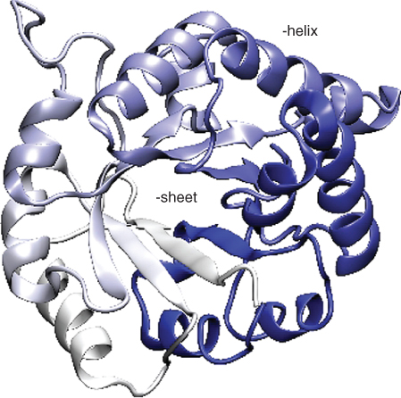
helices and ![]() sheets, along with regions of less well-defined structural elements. Because proteins are such large molecules, and because the secondary structural elements are important parts of the overall structure, most proteins are represented in ways that emphasize the arrangement of secondary structural elements (see Fig. 13.2).
sheets, along with regions of less well-defined structural elements. Because proteins are such large molecules, and because the secondary structural elements are important parts of the overall structure, most proteins are represented in ways that emphasize the arrangement of secondary structural elements (see Fig. 13.2).
Figure 13.2 An ![]() -carbon trace emphasizing the secondary structure of one monomer of the enzyme triose phosphate isomerase (from PDB ID 2YPI). This protein folds into an
-carbon trace emphasizing the secondary structure of one monomer of the enzyme triose phosphate isomerase (from PDB ID 2YPI). This protein folds into an ![]() barrel structure, with a multistrand
barrel structure, with a multistrand ![]() sheet (the thick arrows near the center of the structure) surrounded by
sheet (the thick arrows near the center of the structure) surrounded by ![]() -helical elements. A number of other proteins exhibit this
-helical elements. A number of other proteins exhibit this ![]() barrel structure, despite considerable difference in both their sequence and function.
barrel structure, despite considerable difference in both their sequence and function.
Analysis of protein structures has revealed that many proteins consist of one or more separate domains, which are regions within the protein that fold independently of the remainder of the protein. Protein domains are currently considered to be units of evolution; one major constraint on tolerated mutations is the result of the requirement to maintain the folded structure of the domain.
Comparison of different proteins is crucial to an understanding of the relationships between protein amino acid sequences, protein structure, and protein function. Protein sequence information can be obtained from the genome sequencing projects, and protein sequences can be readily compared. However, many proteins are known to have limited sequence similarity and yet have structures that appear visually similar. This raises the question of how to compare complex 3D structures both quantitatively and in ways that will allow a better understanding of the relationships between their structure and function.
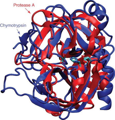
Many proteins exhibit generally similar structures and similar functions. For example, a considerable number of serine protease enzymes have been discovered from species as widely divergent as mammals and bacteria. Although the two proteins shown in Figure 13.3 have very different amino acid sequences, portions of the structure match rather closely. However, in analyzing the structures, it is less clear how important the structural differences are in the subtle differences in function between these proteins. In addition, it is less clear how to best represent the structural differences in a manner that is both consistent and informative.
Figure 13.3 An overlay of two proteins with similar function: protease A from the bacterium Streptomyces griseus (PDB ID 3SGA) and Bos taurus chymotrypsin (PDB ID 1YPH). The two proteins share limited sequence identity (![]() 20%), but similar catalytic mechanisms, and considerable structural similarity, especially in the core of the protein. In contrast, another protein, subtilisin from Bacillus amyloliquefaciens, also exhibits a similar catalytic mechanism but has a very different structure.
20%), but similar catalytic mechanisms, and considerable structural similarity, especially in the core of the protein. In contrast, another protein, subtilisin from Bacillus amyloliquefaciens, also exhibits a similar catalytic mechanism but has a very different structure.
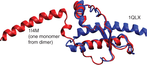
Another example of the importance of structure is provided by the prion proteins (see Fig. 13.4). Prions are monomeric proteins normally found on the surface of a variety of cells; however, these proteins are capable of undergoing an incompletely understood conformational change that results in oligomerization, with lethal effects to the affected individual. The spongiform encephalopathy diseases are one of a significant number of diseases caused by protein misfolding. An improved understanding of protein structure and protein folding processes might allow intervention in disease processes that are currently untreatable. In addition, many genetic disorders result from altered protein structure and function. While it is apparent that the changes in one of a small number of residues within a large protein cause disease, only a better understanding of the elaboration of sequence information into an overall structure will allow insight into possible approaches for treatment.
Figure 13.4 The same protein in two different conformations: a fragment from the human prion protein. The 1I4M structure is part of a dimer, which may represent a stage in the structural transformation from the largely helical protein shown here to the toxic ![]() -sheet conformation thought to cause the lethal spongiform encephalopathy diseases such as Creutzfeldt–Jakob disease and kuru.
-sheet conformation thought to cause the lethal spongiform encephalopathy diseases such as Creutzfeldt–Jakob disease and kuru.
A final purpose of studying protein structure is to allow the design of novel proteins. Enzymes are phenomenal catalysts, which generally exhibit both high reaction rates and high levels of specificity. While biological enzymes catalyze a large range of reactions, no enzymes exist to catalyze many industrially useful reactions. The ability to design new enzyme mechanisms is extremely attractive as a method for carrying out reactions at higher rates, with less expense from heating costs and waste product formation. Current methods for protein design are inefficient and essentially entirely empirical and are largely limited to minor alterations to existing proteins.
We have an increasing database of protein structures; however, we still lack a full understanding of how protein sequence, structure, and function are related. Comparing the structures of existing proteins of different sequences provides important data that will likely lead to an improved understanding of the mechanisms by which existing protein sequences give rise to their corresponding functional protein structures.
13.3 Mathematical Frameworks
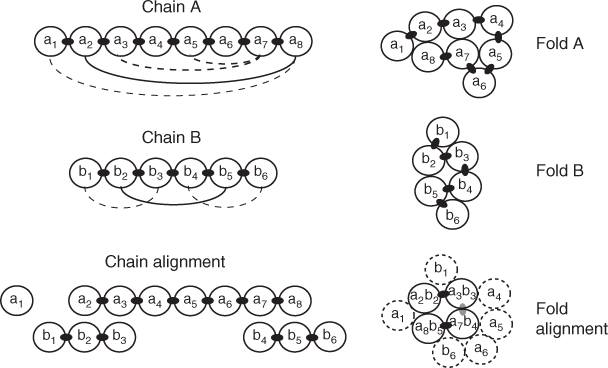
The two main mathematical frameworks studied in the protein alignment literature are the contact map overlap (CMO) problem and the largest common point set (LCP) problem under bottleneck distance constraint [17]. Figure 13.5 illustrates a 2D version of each framework.
Figure 13.5 A 2D depiction of protein alignment. Chain A collapses into fold A, creating long-range contact depicted by arcs on chain A. Likewise, chain B collapses into fold B. Then a rigid-body transformation, in this case a vertical translation, superimposes folds A and B to create a fold alignment. In the CMO problem, the arcs on chains A and B are aligned directly (solid arcs) without reference to the superimposed folds. (The consecutive chain contacts are not considered.) In the LCP problem, the superimposed folds determine the chain alignment.
Let ![]() and
and ![]() be the sets of C
be the sets of C![]() atom coordinates of two proteins, proteins A and B, that we wish to align. (These are the carbon atoms in Fig. 13.1 that bind to the sidechains.) For a given distance cutoff value
atom coordinates of two proteins, proteins A and B, that we wish to align. (These are the carbon atoms in Fig. 13.1 that bind to the sidechains.) For a given distance cutoff value ![]() , define
, define ![]() and
and ![]() to be the sets of edges in the contact graphs of proteins A and B, respectively. (Edges are represented by arcs in Fig. 13.5.) Define
to be the sets of edges in the contact graphs of proteins A and B, respectively. (Edges are represented by arcs in Fig. 13.5.) Define ![]() to be a bijection (one-to-one, onto map) from a subset
to be a bijection (one-to-one, onto map) from a subset ![]() to a subset
to a subset ![]() . Define
. Define ![]() to be a rigid-body transformation of the fold of protein B. (In Figure 13.5,
to be a rigid-body transformation of the fold of protein B. (In Figure 13.5, ![]() is simply a translation of fold B onto fold A.) Then solve the two problems as follows:
is simply a translation of fold B onto fold A.) Then solve the two problems as follows:
Goldman et al. [9] proved that the CMO problem is NP-hard. Caprara et al. [6] apply linear integer programming methods to obtain exact solutions to the CMO problem for proteins that are similar to one another. Their methods have been improved significantly by Andonov et al. [1] (see Section 13.4). By imposing a proximity requirement for aligned residues and employing packing constraints satisfied by actual protein folds, Xu et al. [25] and Li and Ng [17] have developed polynomial time approximation schemes for the CMO problem. The CMO problem is discussed further in Section 13.4.
The LCP problem appears to be easier to solve than the CMO problem. The LCP problem is more geometric in character, whereas the CMO problem is graph-theoretic in nature. A possible disadvantage of the LCP problem, however, is that it treats proteins as rigid objects. In reality proteins are quite flexible. Hasegawa and Holm [10] claim that alignment methods that allow for flexibility give the most biologically meaningful results.
The main ideas used to develop a polynomial time algorithm for the LCP problem are due to Kolodny and Linial [13] and Poleksic [19, 20]. We describe next a polynomial time algorithm for solving the LCP problem. The basic ideas were developed by Kolodny and Linial [13] and extended by Poleksic [20]. Although their analysies [13, 20] pertain to the 3D alignment problem, here, for simplicity of exposition, we describe the algorithm for the 2D alignment problem.
In two dimensions, we can parametrize rigid-body transformations by ![]() as
as
![]()
where ![]() is the coordinates of a C
is the coordinates of a C![]() atom in protein fold B. For a prescribed distance cutoff value,
atom in protein fold B. For a prescribed distance cutoff value, ![]() , and for a given rigid-body transformation
, and for a given rigid-body transformation ![]() , define
, define ![]() to be the largest subset of
to be the largest subset of ![]() for which there exists a bijection
for which there exists a bijection ![]() such that
such that
![]()
The set ![]() and the bijection
and the bijection ![]() can easily be computed in
can easily be computed in ![]() time by applying dynamic programming, see Section 13.4 for the score matrix
time by applying dynamic programming, see Section 13.4 for the score matrix ![]() , where
, where
The solution to the LCP problem is then given by ![]() .
.
A key observation by Kolodny and Linial [13] is that only a finite set of rigid-body transformations needs to be considered in order to optimize commonly used alignment scoring functions. To demonstrate this, first observe that only the compact subset, ![]() of rigid-body transformations needs to be considered because if protein
of rigid-body transformations needs to be considered because if protein ![]() is translated by
is translated by ![]() or
or ![]() , where
, where ![]() is sufficiently large,
is sufficiently large, ![]() will be the empty set since proteins
will be the empty set since proteins ![]() and
and ![]() will have no points in common. Since
will have no points in common. Since ![]() is continuous and
is continuous and ![]() is compact,
is compact, ![]() is uniformly continuous on
is uniformly continuous on ![]() . Uniform continuity implies that there exists a
. Uniform continuity implies that there exists a ![]() such that for any
such that for any ![]() and
and ![]() satisfying
satisfying ![]() we have that
we have that ![]() for all
for all ![]() . Now, consider the open balls
. Now, consider the open balls ![]() where
where ![]() . The open balls
. The open balls ![]() cover
cover ![]() , that is,
, that is, ![]() . Since
. Since ![]() is compact, a finite subset of these open balls also covers
is compact, a finite subset of these open balls also covers ![]() ; that is, there exist
; that is, there exist ![]() such that
such that ![]() . Thus, all the rigid-body transformations in the compact set
. Thus, all the rigid-body transformations in the compact set ![]() can be approximated to within a distance of
can be approximated to within a distance of ![]() by the finite set of rigid-body transformations
by the finite set of rigid-body transformations ![]() .
.
The alignment scoring functions considered by Kolodny and Linial [13] must satisfy a Lipschitz condition. Their algorithm only computes an ![]() approximation of the optimal solution. Poleksic [20] extended Kolodny and Linial's approach to the LCP problem. Moreover, Poleksic's extension computes the exact solution to the LCP problem in expected polynomial time
approximation of the optimal solution. Poleksic [20] extended Kolodny and Linial's approach to the LCP problem. Moreover, Poleksic's extension computes the exact solution to the LCP problem in expected polynomial time ![]() for globular proteins of size
for globular proteins of size ![]() [19, 20]. We describe Poleksic's algorithm next.
[19, 20]. We describe Poleksic's algorithm next.
Let ![]() . Also, for
. Also, for ![]() , define the function
, define the function ![]() , where
, where ![]() is the number of elements in
is the number of elements in ![]() . Since
. Since ![]() , there exists an
, there exists an ![]() such that
such that ![]() , which implies
, which implies
![]()
From this inequality, we can conclude that
![]()
because if ![]() and
and ![]() are in contact for cutoff
are in contact for cutoff ![]() , then
, then ![]() and
and ![]() remain in contact for cutoff
remain in contact for cutoff ![]() . We also have that
. We also have that
![]()
Combining these inequalities, we have
![]()
The LCP problem can be solved exactly in a finite number of steps if we can determine an ![]() for which
for which
![]()
since this would imply that ![]() . Poleksic [20] showed that such an
. Poleksic [20] showed that such an ![]() exists for all except a finite set of cutoff values
exists for all except a finite set of cutoff values ![]() as follows. The function
as follows. The function ![]() is a nondecreasing function of
is a nondecreasing function of ![]() having integer values in the range from
having integer values in the range from ![]() to
to ![]() . The function
. The function ![]() is therefore piecewise constant except for possible jump discontinuities at cutoff values
is therefore piecewise constant except for possible jump discontinuities at cutoff values ![]() . If we avoid this finite set of cutoff values, then we can choose an
. If we avoid this finite set of cutoff values, then we can choose an ![]() such that
such that ![]() . The size of the finite set of rigid-body transformations
. The size of the finite set of rigid-body transformations ![]() that we need to search to determine
that we need to search to determine ![]() is determined by how small
is determined by how small ![]() is. The size of
is. The size of ![]() is determined by how close
is determined by how close ![]() is to one of the jump discontinuity points
is to one of the jump discontinuity points ![]() ,
, ![]() . These jump discontinuity points are not known in advance. However, Poleksic [20] provides a proof that the overall expected complexity of the algorithm is polynomial in time.
. These jump discontinuity points are not known in advance. However, Poleksic [20] provides a proof that the overall expected complexity of the algorithm is polynomial in time.
13.3.1 Spectral Methods
Spectral methods have emerged as a new mathematical framework for the protein structure alignment problem. An advantage of spectral methods over CMO methods pointed out by Bhattacharya et al. [4] is that comparisons with spectral methods are based on two residues (one from each protein) rather than the four residues (two from each protein to define an edge) required by CMO methods. Another advantage over CMO pointed out by Lena et al. [15] is that unlike CMO, spectral methods scale well with the size of the distance cutoff parameter ![]() .
.
In 1988, Umeyama [23] published a spectral, polynomial-time algorithm for computing a bijection between two weighted graphs that are isomorphic. The adjacency matrix of each graph is assume to have distinct eigenvalues. Umeyama's algorithm also works well if the graphs are nearly isomorphic. We describe the details of Umeyama's algorithm next.
Let ![]() and
and ![]() be the adjacency matrices of two undirected, weighted graphs with the same number of nodes and distinct eigenvalues. The goal is to determine a permutation matrix
be the adjacency matrices of two undirected, weighted graphs with the same number of nodes and distinct eigenvalues. The goal is to determine a permutation matrix ![]() that minimizes
that minimizes ![]() . Let
. Let ![]() and
and ![]() be the eigensystem decomposition of
be the eigensystem decomposition of ![]() and
and ![]() . It is possible to prove that
. It is possible to prove that
where ![]() and
and ![]() ,
, ![]() , are the ordered eigenvalues of
, are the ordered eigenvalues of ![]() and
and ![]() . Umeyama showed that there exists an orthogonal matrix
. Umeyama showed that there exists an orthogonal matrix ![]() for some diagonal matrix
for some diagonal matrix ![]() , where
, where ![]() has diagonal elements
has diagonal elements ![]() or 1, for which
or 1, for which
For isomorphic graphs, Umeyama proved that ![]() is a permutation matrix
is a permutation matrix ![]() . Moreover,
. Moreover, ![]() can be computed in polynomial time by solving the assignment problem
can be computed in polynomial time by solving the assignment problem
![]()
using the Hungarian algorithm. (The entries of the matrices ![]() and
and ![]() are the absolute values of the entries in
are the absolute values of the entries in ![]() and
and ![]() .) Umeyama also observed that the optimal solution can often be obtained for nonisomorphic graphs by using the solution to the assignment problem above as an initial guess and then applying a local optimization algorithm.
.) Umeyama also observed that the optimal solution can often be obtained for nonisomorphic graphs by using the solution to the assignment problem above as an initial guess and then applying a local optimization algorithm.
Umeyama's algorithm for the graph isomorphism problem does not apply directly to the protein structure alignment problem, which is a subgraph isomorphism problem. In other words, Umeyama's algorithm cannot handle insertions and deletions. In addition, the weighted graphs of protein structures may not be similar to one another, a requirement for Umeyama's algorithm to work reliably.
Bhattacharya et al. [4] attempt to overcome the limitations of Umeyama's algorithm by considering local alignments to identify similar neighborhoods of the same size and then piecing these neighborhoods together. Rather than apply Umeyama's algorithm directly, Bhattacharya et al. normalize each eigenvector by the size of the protein and then compare the eigenvectors without taking absolute values. (Like Umeyama, they do not use the eigenvalues in their algorithm.) A complication arising in the approach used by Bhattacharya et al. is the fact that the eigenvector decomposition of an adjacency matrix does not specify an orientation of the eigenvectors. In other words, if ![]() is an eigenvector, so is
is an eigenvector, so is ![]() . This requires
. This requires ![]() eigenvector orientations to be checked, where
eigenvector orientations to be checked, where ![]() equals the number of eigenvectors compared. The time complexity of the resulting algorithm, called Matchprot, is
equals the number of eigenvectors compared. The time complexity of the resulting algorithm, called Matchprot, is ![]() . Bhattacharya et al. point out that empirical observations suggest that
. Bhattacharya et al. point out that empirical observations suggest that ![]() eigenvectors is sufficient for good results. However, Matchprot has difficulty with alignments involving large insertions and deletions.
eigenvectors is sufficient for good results. However, Matchprot has difficulty with alignments involving large insertions and deletions.
Lena et al. [15] introduced a spectral algorithm called Al-Eigen. Unlike Matchprot, Al-Eigen uses a global alignment. Al-Eigen scales eigenvectors by the square root of the corresponding eigenvalues. Like Matchprot, Al-Eigen searches through the ![]() orientations of the
orientations of the ![]() eigenvectors it compares, starting with comparing just one eigenvector from each protein, up to
eigenvectors it compares, starting with comparing just one eigenvector from each protein, up to ![]() eigenvectors. The complexity of Al-Eigen is
eigenvectors. The complexity of Al-Eigen is ![]() .
.
In this section we have tersely reviewed the primary mathematical models associated with optimally aligning protein structures. The intent of the CMO, the LCP, and the spectral frameworks is to discern biologically relevant alignments between two proteins. Each paradigm has advantages and disadvantages, and continued research is important. The algorithmic complexity and resulting solution times were substantial enough that, until quite recently, undertaking the task of completing numerous pairwise comparisons was a weighty computational burden. However, a host of modern algorithms is emerging that hasten the comparison procedure. These are discussed in the next section.
13.4 More Recent Advances with Database Queries
Protein databases contain tens of thousands of structures and continue to grow. One of the research fronts in computational biology is the design of algorithms that can efficiently search and organize these databases. For example, a researcher may want to find those proteins whose structure is similar to one under investigation, or may want to navigate a database by functionally similar proteins. Such queriesrequire comparisons against an entire database. As protein databases grow, undertaking these numerous comparisons requires efficient and accurate comparison algorithms.
We review three methods that are designed for making efficient structural comparisons: (1) a geometric approach that encodes each residue with angle and distance information called globa structure superposition of proteins (GOSSIP) [12] (2) a spectral approach called EIGAS that assigns each residue an eigenvalue associated with a high-dimensional feature [22], and (3) a solution procedure to the CMO problem called A_purva [1]. While these methods represent protein chains differently, they share the common algorithmic solution procedure of dynamic programming (DP). The emerging literature on protein structure alignment points to the important role that DP is fulfilling as an efficient algorithmic framework. Our specific goal here is to highlight this observation and develop the use of DP in each of these alignment procedures.
Dynamic programming was invented by Bellman in the 1940s [3], and its use in biological applications began in 1970 [18]. The discrete version we consider calculates an optimal match between two sequences, say, ![]() and
and ![]() . The algorithm requires that each possible match be scored, and we let
. The algorithm requires that each possible match be scored, and we let ![]() be the score associated with matching element
be the score associated with matching element ![]() of the first sequence with element
of the first sequence with element ![]() of the second. Dynamic programming follows a recursion to calculate an optimal match between the two sequences
of the second. Dynamic programming follows a recursion to calculate an optimal match between the two sequences
where ![]() is a gap penalty. The gap penalty can depend on whether a gap is being initiated or continued; in the former the penalty is called a gap opening penalty and in the latter, a gap extension penalty. Completing this recursion over
is a gap penalty. The gap penalty can depend on whether a gap is being initiated or continued; in the former the penalty is called a gap opening penalty and in the latter, a gap extension penalty. Completing this recursion over ![]() and
and ![]() calculates the optimal value of the matching, and backtracing the optimal iterations lists the optimal matching. The optimal match depends not only on the scoring matrix
calculates the optimal value of the matching, and backtracing the optimal iterations lists the optimal matching. The optimal match depends not only on the scoring matrix ![]() but also on the penalties to open and continue a gap, and hence, the use of DP to optimally align sequences requires parameter tuning. The computational complexity of calculating an optimal matching is
but also on the penalties to open and continue a gap, and hence, the use of DP to optimally align sequences requires parameter tuning. The computational complexity of calculating an optimal matching is ![]() , showing that DP is an efficient polynomial algorithm.
, showing that DP is an efficient polynomial algorithm.
The coordinates of the C![]() atoms of each residue are used to describe the protein in each of the techniques presented below. Because of the lack of an absolute coordinate system, a protein is commonly abstracted into pairwise comparisons between C
atoms of each residue are used to describe the protein in each of the techniques presented below. Because of the lack of an absolute coordinate system, a protein is commonly abstracted into pairwise comparisons between C![]() atoms, which provides a coordinate and rotation free description of the protein. Each of A_purva, GOSSIP, and EIGAS assigns different information to each C
atoms, which provides a coordinate and rotation free description of the protein. Each of A_purva, GOSSIP, and EIGAS assigns different information to each C![]() atom, and hence, each imposes a different pairwise relationship between residues. In what follows, we briefly describe each technique soas to highlight the similarities and dissimilarities between the algorithms. In particular, we show how to construct the scoring matrices used for DP so that each method is seen as an application of DP applied to sequence similarity.
atom, and hence, each imposes a different pairwise relationship between residues. In what follows, we briefly describe each technique soas to highlight the similarities and dissimilarities between the algorithms. In particular, we show how to construct the scoring matrices used for DP so that each method is seen as an application of DP applied to sequence similarity.
13.4.1 GOSSIP
The GOSSIP algorithm uses DP with a scoring matrix created by local 3D geometry. A residue is encoded with eight characteristics that depend on a parameter ![]() that defines the local geometry. The characteristics for residue
that defines the local geometry. The characteristics for residue ![]() depend on the polygon created by residues
depend on the polygon created by residues ![]() ,
, ![]() ,
, ![]() , and
, and ![]() . Five of the characteristics are distances, and we use
. Five of the characteristics are distances, and we use ![]() to denote the Euclidean distance between the C
to denote the Euclidean distance between the C![]() atoms of residues
atoms of residues ![]() and
and ![]() . The characteristics are
. The characteristics are
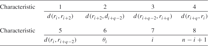
The angle ![]() is created by the line segments
is created by the line segments ![]() and
and ![]() , where
, where ![]() is the centroid of the protein structure and
is the centroid of the protein structure and ![]() is the number of residues in the protein chain. See Figure 13.6 for an example. All but the last
is the number of residues in the protein chain. See Figure 13.6 for an example. All but the last ![]() residues are encoded.
residues are encoded.
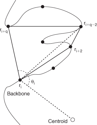
Figure 13.6 Residue ![]() is characterized by lengths of a polygon, the length of a diagonal, the angle
is characterized by lengths of a polygon, the length of a diagonal, the angle ![]() , and two indices.
, and two indices.
The score assigned to matching residue ![]() of the first protein to residue
of the first protein to residue ![]() of the second is
of the second is
![]()
where the coefficients ![]() and
and ![]() are experimentally decided. DP is applied to the scoring matrix
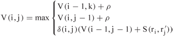
are experimentally decided. DP is applied to the scoring matrix ![]() , but with a few adaptations. First, an indicator function
, but with a few adaptations. First, an indicator function ![]() is used to decide if the characteristics of residues
is used to decide if the characteristics of residues ![]() and
and ![]() are similar enough to consider a match. Each characteristic is compared, and agreement is decided based on a threshold value that is characteristic dependent. If enough characteristics agree, then
are similar enough to consider a match. Each characteristic is compared, and agreement is decided based on a threshold value that is characteristic dependent. If enough characteristics agree, then ![]() , but if not
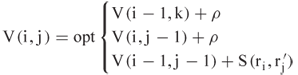
, but if not ![]() . This adaptation alters the recursion in (13.1) to
. This adaptation alters the recursion in (13.1) to
A second adaptation is that ![]() is not calculated if the difference between
is not calculated if the difference between ![]() and
and ![]() exceeds a threshold indicating the maximum number of gaps allowed in a match. GOSSIP further limits the number of the protein chains that are compared by associating with each chain a collection of chains of similar lengths.
exceeds a threshold indicating the maximum number of gaps allowed in a match. GOSSIP further limits the number of the protein chains that are compared by associating with each chain a collection of chains of similar lengths.
Numerical work for GOSSIP is promising. Two datasets described by Kifer et al. [12] were used for testing, one containing 2,930 protein structures from CATH and one containing 3,613 structures from Astral. An all-against-all comparison requires 4,290,985 alignments in the CATH dataset and 6,525,078 comparisons in the Astral dataset. To gauge the effectiveness of GOSSIP, ![]() proteins from the CATH dataset and
proteins from the CATH dataset and ![]() from the Astral dataset were selected, and all-against-all comparisons were made on these smaller datasets. Runtimes were then scaled to the larger datasets. The GOSSIP adaptations to DP were estimated to complete all pairwise comparisons in the large datasets in the range from 9 (17.3) h to 5.1 (9.1) min on CATH (Astral), depending on how similar the lengths of the protein chains needed to be to consider an alignment. The longest runtimes were for comparisons in which the chain lengths need to be within only
from the Astral dataset were selected, and all-against-all comparisons were made on these smaller datasets. Runtimes were then scaled to the larger datasets. The GOSSIP adaptations to DP were estimated to complete all pairwise comparisons in the large datasets in the range from 9 (17.3) h to 5.1 (9.1) min on CATH (Astral), depending on how similar the lengths of the protein chains needed to be to consider an alignment. The longest runtimes were for comparisons in which the chain lengths need to be within only ![]() of each other, and the shortest times required the chain lengths to be within
of each other, and the shortest times required the chain lengths to be within ![]() of each other. The accuracy of the method lies between the results of MultiProt [21] and YAKUSA [7], and while MultiProt better identifies structural similarity, it requires several hundred hours of computational time. GOSSIP bests YAKUSA's results while comparing reasonably with regard to run time.
of each other. The accuracy of the method lies between the results of MultiProt [21] and YAKUSA [7], and while MultiProt better identifies structural similarity, it requires several hundred hours of computational time. GOSSIP bests YAKUSA's results while comparing reasonably with regard to run time.
13.4.2 Eigensystem Alignment with a Spectrum
As with the other methods described in this section, the central theme of aligning protein chains by EIGensystem Alignment with the Spectrum (EIGAS) is to align the residues so that the matching is as similar as possible with regard to a measure of intra-similarity between the residues of the individual proteins. EIGAS uses a scaled version of the Euclidean distance between the C![]() atoms of any two residues, a measure called smooth contact. A smooth-contact matrix
atoms of any two residues, a measure called smooth contact. A smooth-contact matrix ![]() has as its
has as its ![]() th element the smooth contact between residues
th element the smooth contact between residues ![]() and
and ![]() ,
,
![]()
where ![]() is the Euclidean distance between the C
is the Euclidean distance between the C![]() atoms of residues
atoms of residues ![]() and
and ![]() . Euclidean distances less than the cutoff parameter
. Euclidean distances less than the cutoff parameter ![]() are scaled linearly between the maximum smooth-contact value of 1, which occurs if
are scaled linearly between the maximum smooth-contact value of 1, which occurs if ![]() , and the minimum value of 0, which occurs if the distance between the residues exceeds
, and the minimum value of 0, which occurs if the distance between the residues exceeds ![]() . The smooth-contact measure is an assessment of the proximity of the residues. So the smooth contact between a residue and itself is 1. If
. The smooth-contact measure is an assessment of the proximity of the residues. So the smooth contact between a residue and itself is 1. If ![]() is small, then the smooth contact between most residues is zero, but if
is small, then the smooth contact between most residues is zero, but if ![]() is large, then more values are nonzero.
is large, then more values are nonzero.
Smooth-contact matrices have the favorable mathematical property that they are positive definite, that is, that all eigenvalues are positive, for suitably small ![]() values. This follows from the fact that the diagonal elements are independent of the value of
values. This follows from the fact that the diagonal elements are independent of the value of ![]() since a Cα atom is always in contact with itself, whereas the off-diagonal elements can be made arbitrarily small as
since a Cα atom is always in contact with itself, whereas the off-diagonal elements can be made arbitrarily small as ![]() decreases. Hence the sum of the off-diagonal elements of any row is guaranteed to be less than the diagonal element itself for sufficiently small
decreases. Hence the sum of the off-diagonal elements of any row is guaranteed to be less than the diagonal element itself for sufficiently small ![]() , a property called diagonal dominance. A well-known result in linear algebra is that a diagonally dominant matrix is positive definite. The positive definite property guarantees that a smooth-contact matrix can be factored as
, a property called diagonal dominance. A well-known result in linear algebra is that a diagonally dominant matrix is positive definite. The positive definite property guarantees that a smooth-contact matrix can be factored as
13.2 ![]()
where the columns of ![]() form an orthonormal set of eigenvectors of
form an orthonormal set of eigenvectors of ![]() and
and ![]() is a diagonal matrix of the positive eigenvalues. Moreover, a smooth-contact matrix imposes an inner product, and subsequently a norm and a metric, on
is a diagonal matrix of the positive eigenvalues. Moreover, a smooth-contact matrix imposes an inner product, and subsequently a norm and a metric, on ![]() , where
, where ![]() is the number of residues in the protein chain. So, each protein chain coincides with a geometric rendering of
is the number of residues in the protein chain. So, each protein chain coincides with a geometric rendering of ![]() .
.
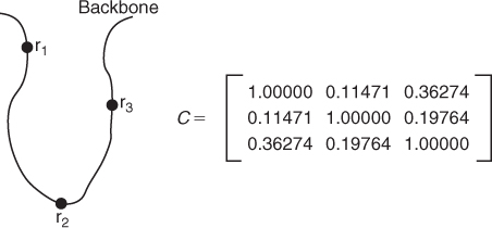
To illustrate the mathematical and geometric properties induced by a smooth-contact matrix, we consider a three-residue protein chain whose smooth-contact matrix is located in Figure 13.7. The inner product of the vectors ![]() and
and ![]() induced by the smooth-contact matrix is
induced by the smooth-contact matrix is ![]() , which has the following properties:
, which has the following properties:
 is the norm of
  relative to
  .
. is the cosine of the angle between
  and
and  .
. is the distance between
  and
and  relative to
  .
.
The inner product supports an embedding of the residues in an ![]() -dimensional space so that the smooth contact between any two residues is the result of an inner product calculation. Let the first residue be associated with
-dimensional space so that the smooth contact between any two residues is the result of an inner product calculation. Let the first residue be associated with ![]() , the second with
, the second with ![]() , and so on. Then
, and so on. Then ![]() , which is the smooth contact between residues
, which is the smooth contact between residues ![]() and
and ![]() , for example,
, for example, ![]() for the smooth-contact matrix in Figure 13.7.
for the smooth-contact matrix in Figure 13.7.
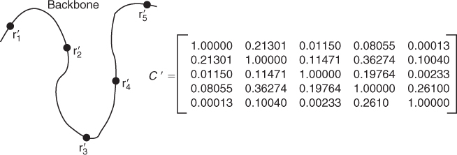
Figure 13.7 The path of the backbone indicates that the Euclidean distances between residues 1 and 3 and between 2 and 3 are shorter than the distance between residues 1 and 2. This is seen in the smooth-contact matrix since both ![]() and
and ![]() , both of which are greater than
, both of which are greater than ![]() .
.
The vector space ![]() with the inner product
with the inner product ![]() is called a contact space, and the geometry induced by
is called a contact space, and the geometry induced by ![]() is, in some sense, a “skewed” Euclidean geometry. As an illustration we note that a sphere is the collection of unit length vectors, which in contact space means that
is, in some sense, a “skewed” Euclidean geometry. As an illustration we note that a sphere is the collection of unit length vectors, which in contact space means that ![]() is on the sphere only if
is on the sphere only if ![]() . Such a collection is an ellipsoid because the metric is scaled by
. Such a collection is an ellipsoid because the metric is scaled by ![]() . The unit ellipsoid with respect to the contact matrix in Figure 13.7 is depicted in Figure 13.8. The residues are represented by the thick dark vectors
. The unit ellipsoid with respect to the contact matrix in Figure 13.7 is depicted in Figure 13.8. The residues are represented by the thick dark vectors ![]() ,
, ![]() , and
, and ![]() , which lie along the standard axes. The angle between
, which lie along the standard axes. The angle between ![]() and
and ![]() is not as it appears in the figure. For example, in Euclidean geometry the angle between
is not as it appears in the figure. For example, in Euclidean geometry the angle between ![]() and
and ![]() is 90°, but in contact space the angle is
is 90°, but in contact space the angle is ![]() . Also, in Euclidean geometry the distance between between
. Also, in Euclidean geometry the distance between between ![]() and
and ![]() is
is ![]() , but in contact space the distance is
, but in contact space the distance is ![]() .
.
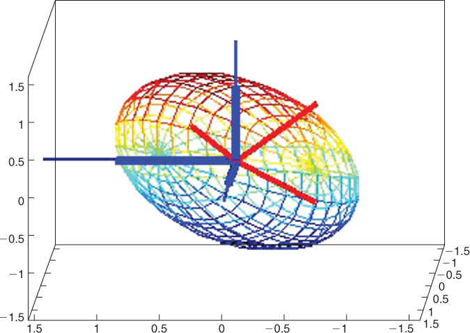
Figure 13.8 The ellipsoid is the collection of all unit length vectors with respect to the contact matrix in Figure 13.7. The thick dark vectors represent the residues and are ![]() (pointing to the left),
(pointing to the left), ![]() (pointing out from the page), and
(pointing out from the page), and ![]() (pointing upward). The thin vectors are the orthonormal eigenvectors that form the columns of
(pointing upward). The thin vectors are the orthonormal eigenvectors that form the columns of ![]() in Equation (13.2). The eigenvectors lie along the principal axes of the ellipsoid, and the length of each axis is
in Equation (13.2). The eigenvectors lie along the principal axes of the ellipsoid, and the length of each axis is ![]() .
.
The motivation behind EIGAS is that each protein is associated with an ![]() -dimensional geometry, and this perspective allows the problem of aligning protein structures to be restated as a question of optimally aligning the geometries of contact spaces. However, contact spaces vary in dimension just as protein chains vary in length, and the algorithmic design question is to create a method of matching the residues so that the lower-dimensional geometries of the two contact spaces are as similar as possible.
-dimensional geometry, and this perspective allows the problem of aligning protein structures to be restated as a question of optimally aligning the geometries of contact spaces. However, contact spaces vary in dimension just as protein chains vary in length, and the algorithmic design question is to create a method of matching the residues so that the lower-dimensional geometries of the two contact spaces are as similar as possible.
Contact geometries are defined by the eigenvectors and eigenvalues, which give the direction and length of the unit ellipsoid's principal axes. Moreover, the eigenvectors are linear combinations of the ![]() vectors. So, in terms of the protein, each eigenvector represents a weighted sum of the residues in contact space. In some research communities these weighted sums would be called “features” of the protein. Each residue is associated with its nearest eigenvector and is assigned its corresponding eigenvalue. Formally, residue
vectors. So, in terms of the protein, each eigenvector represents a weighted sum of the residues in contact space. In some research communities these weighted sums would be called “features” of the protein. Each residue is associated with its nearest eigenvector and is assigned its corresponding eigenvalue. Formally, residue ![]() is assigned the eigenvalue
is assigned the eigenvalue ![]() , where the associated eigenvector
, where the associated eigenvector ![]() of the smooth-contact matrix solves
of the smooth-contact matrix solves
![]()
where ![]() denotes the eigenvectors that comprise the columns of
denotes the eigenvectors that comprise the columns of ![]() and
and ![]() from Equation (13.2). This eigenvalue assignment associates each residue with one of the principal axes of the ellipsoid defined by the smooth-contact map. A matching of the residues between the protein chains is scored by comparing the eigenvalues associated with the corresponding principal axes.
from Equation (13.2). This eigenvalue assignment associates each residue with one of the principal axes of the ellipsoid defined by the smooth-contact map. A matching of the residues between the protein chains is scored by comparing the eigenvalues associated with the corresponding principal axes.
Consider the problem of matching the protein chain in Figure 13.7 with the chain in Figure 13.9. The middle three residues of the chain in Figure 13.9 are in the same configuration as the residues inFigure 13.7, and one would expect an alignment technique to match ![]() with
with ![]() ,
, ![]() with
with ![]() , and
, and ![]() with
with ![]() . The eigenvalues of the smooth-contact matrix in Figure 13.7 are
. The eigenvalues of the smooth-contact matrix in Figure 13.7 are ![]() , 0.91, and
, 0.91, and ![]() , and the eigenvalues of the smooth-contact matrix in Figure 13.9 are
, and the eigenvalues of the smooth-contact matrix in Figure 13.9 are ![]() ,
, ![]() ,
, ![]() ,
, ![]() , and
, and ![]() . Assigning the residues the eigenvalues of their nearest eigenspaces leads to the matching problem depicted below:
. Assigning the residues the eigenvalues of their nearest eigenspaces leads to the matching problem depicted below:
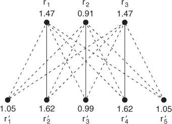
Figure 13.9 Residues ![]() ,
, ![]() , and
, and ![]() are in the same geometric configuration with
are in the same geometric configuration with ![]() ,
, ![]() , and
, and ![]() , respectively, in Figure 13.7
, respectively, in Figure 13.7
The optimal three-residue matching is shown by the solid edges. The optimal value is the combined eigenvalue difference, ![]() , which is the lowest possible among all matchings of three residues. Note that this is the anticipated alignment.
, which is the lowest possible among all matchings of three residues. Note that this is the anticipated alignment.
The value of matching residue ![]() with residue
with residue ![]() is estimated by
is estimated by ![]() . If the eigenvalues are similar, then the principal axes of the unit ellipsoids associated with the residues are of approximately the same length. Hence the contact geometries are similar along these particular axes. EIGAS uses the scoring matrix
. If the eigenvalues are similar, then the principal axes of the unit ellipsoids associated with the residues are of approximately the same length. Hence the contact geometries are similar along these particular axes. EIGAS uses the scoring matrix ![]() and DP to find an optimal matching between the residues. EIGAS was reported [22] to correctly identify the SCOP classification of the Skolnick40 dataset by completing all 780 comparisons in about
and DP to find an optimal matching between the residues. EIGAS was reported [22] to correctly identify the SCOP classification of the Skolnick40 dataset by completing all 780 comparisons in about ![]() s. On Proteus300 EIGAS completed all
s. On Proteus300 EIGAS completed all ![]() comparisons in about
comparisons in about ![]() h. The best results in terms of quality were achieved with
h. The best results in terms of quality were achieved with ![]() Å and a gap penalty of
Å and a gap penalty of ![]() . More recent results [11] show that EIGAS can complete all
. More recent results [11] show that EIGAS can complete all ![]() comparisons in
comparisons in ![]() seconds if the DP is coded in C
seconds if the DP is coded in C![]() and the computational effort is distributed over eight cores. This more recent numerical work shows that if
and the computational effort is distributed over eight cores. This more recent numerical work shows that if ![]() Å, the gap opening penalty is
Å, the gap opening penalty is ![]() , and the gap extension penalty is
, and the gap extension penalty is ![]() , then EIGAS correctly identifies the SCOP classifications of Proteus300 (perfect classifications were reported for many parameter combinations).
, then EIGAS correctly identifies the SCOP classifications of Proteus300 (perfect classifications were reported for many parameter combinations).
13.4.3 A_purva
As is often the case in applied mathematics, the concept of structure can be represented in terms of graph theory, and this is the manner in which contact map overlap (CMO) is derived. The backbone of each protein chain is represented as a graph, say, ![]() . The vertices in
. The vertices in ![]() represent the C
represent the C![]() atoms, and two C
atoms, and two C![]() atoms are adjacent, meaning that they form an edge in
atoms are adjacent, meaning that they form an edge in ![]() , if the distance between them satisfies a contact criteria. For example, if
, if the distance between them satisfies a contact criteria. For example, if ![]() , then residues
, then residues ![]() and
and ![]() are in contact and
are in contact and ![]() induces an edge in
induces an edge in ![]() . We let
. We let ![]() be the index set
be the index set ![]() and
and ![]() be the collection of edges
be the collection of edges ![]() such that
such that ![]() satisfies the contact criteria. A_purva [1] uses an upper bound of
satisfies the contact criteria. A_purva [1] uses an upper bound of ![]() Å, and edges for consecutive residues along the protein backbone are not permitted. If we let
Å, and edges for consecutive residues along the protein backbone are not permitted. If we let ![]() form a binary matrix with a value of
form a binary matrix with a value of ![]() if residues
if residues ![]() and
and ![]() satisfy the contact criteria, then we have represented the protein chain as a graph associated with this adjacency matrix (see Fig. 13.10).
satisfy the contact criteria, then we have represented the protein chain as a graph associated with this adjacency matrix (see Fig. 13.10).
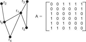
Figure 13.10 A graphical representation of a protein chain of six residues along with its adjacency matrix.
The goal of CMO is to optimize a pairing between the graphical representations of the two proteins, meaning that we want to pair residues so that their contact structures match as well as possible. This question is similar to the classic NP-hard problem of finding a maximum induced subgraph, which is to find the largest possible subgraph of one graph that is a subgraph of the other. However, CMO adds the constraint that the sequential ordering of the nodes must be preserved in the vertex matching. For example, if ![]() of the first protein is matched with
of the first protein is matched with ![]() of the second, then
of the second, then ![]() of the first protein cannot be matched to
of the first protein cannot be matched to ![]() of the second since this would violate the linear ordering inherited from a protein's backbone. Residue
of the second since this would violate the linear ordering inherited from a protein's backbone. Residue ![]() could be matched to any
could be matched to any ![]() of the second protein as long as
of the second protein as long as ![]() .
.
To accomplish the residue matching, the graphs of two proteins are joined to create a bipartite graph. Let ![]() and
and ![]() be the graphs of two proteins and
be the graphs of two proteins and ![]() and
and ![]() be their respective adjacency matrices. Form the complete bipartite graph between the two vertex sets, meaning that every possible edge between
be their respective adjacency matrices. Form the complete bipartite graph between the two vertex sets, meaning that every possible edge between ![]() and
and ![]() is included. The edge sets
is included. The edge sets ![]() and
and ![]() are used to weight every possible pair of matches, indexed by
are used to weight every possible pair of matches, indexed by ![]() to indicate that
to indicate that ![]() of the first protein is matched with
of the first protein is matched with ![]() of the second and that
of the second and that ![]() of the first is matched with
of the first is matched with ![]() of the second. Each
of the second. Each ![]() is assigned the product of the corresponding elements of the adjacency matrices:
is assigned the product of the corresponding elements of the adjacency matrices:

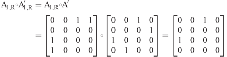
We say that the paired residue matches ![]() and
and ![]() share a common contact provided that
share a common contact provided that ![]() is
is ![]() . As an example, if we are trying to align the protein depicted in Figure 13.10 with a four-residue protein in which the only contacts are between
. As an example, if we are trying to align the protein depicted in Figure 13.10 with a four-residue protein in which the only contacts are between ![]() and
and ![]() and between
and between ![]() and
and ![]() , then
, then ![]() but
but ![]() . A schematic is depicted in Figure 13.11.
. A schematic is depicted in Figure 13.11.
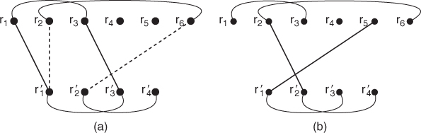
Figure 13.11 Diagram (a) depicts two possible pairs of matchings between two proteins. The pair depicted with solid lines is weighted with a one since ![]() is in contact with
is in contact with ![]() and
and ![]() is in contact with
is in contact with ![]() . The pair depicted by dashed lines is weighted with a zero since
. The pair depicted by dashed lines is weighted with a zero since ![]() is not in contact with
is not in contact with ![]() . Note that not all edges from Figure 13.10 are shown for the top protein. Diagram (b) shows a pairing that would not be allowed since it violates the residue ordering imposed by the proteins' backbones.
. Note that not all edges from Figure 13.10 are shown for the top protein. Diagram (b) shows a pairing that would not be allowed since it violates the residue ordering imposed by the proteins' backbones.
The bipartite weights are used to score matchings between the residue sets by adding all possible weights in the matching. If ![]() is matched with
is matched with ![]() , for
, for ![]() , in the example above, then this matching has a contact score of
, in the example above, then this matching has a contact score of
![]()
This value indicates that the only overlap of this residue matching is due to the fact that matching ![]() to
to ![]() and
and ![]() to
to ![]() yields a common contact. In matrix terms, the score is half of
yields a common contact. In matrix terms, the score is half of ![]() , where
, where ![]() denotes the residues from the first protein;
denotes the residues from the first protein; ![]() , the residues from the second protein; the set subscripts, the submatrices whose rows and columns are listed in the sets; and
, the residues from the second protein; the set subscripts, the submatrices whose rows and columns are listed in the sets; and ![]() , the Hadamard (elementwise) product. The 1-norm is the elementwise norm and not the operator norm. To see the preceding calculation in this matrix form, let
, the Hadamard (elementwise) product. The 1-norm is the elementwise norm and not the operator norm. To see the preceding calculation in this matrix form, let ![]() , which gives
, which gives
As above, the only nonzero elements result from residues ![]() and
and ![]() being in contact in the first protein and residues
being in contact in the first protein and residues ![]() and
and ![]() being in contact in the second. The symmetry of the adjacency matrices doubles the score. The matrix description shows that we are looking for ordered index sets of the residues from both proteins so that the elementwise product of the resulting adjacency submatrices has as many ones as possible.
being in contact in the second. The symmetry of the adjacency matrices doubles the score. The matrix description shows that we are looking for ordered index sets of the residues from both proteins so that the elementwise product of the resulting adjacency submatrices has as many ones as possible.
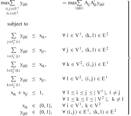
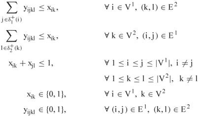
The combinatorial problem of maximizing the contact overlap can be stated as a binary optimization problem. For the ![]() th residue in
th residue in ![]() , with
, with ![]() indicating either the first or second protein, let
indicating either the first or second protein, let ![]() and
and ![]() . We let
. We let ![]() be a binary variable indicating that if we match
be a binary variable indicating that if we match ![]() of the first protein with
of the first protein with ![]() of the second and
of the second and ![]() of the first with
of the first with ![]() of the second. We also let
of the second. We also let ![]() be a binary variable indicating if
be a binary variable indicating if ![]() of the first protein is matched with
of the first protein is matched with ![]() of the second. With this notation, the standard formulation of the CMO problem is
of the second. With this notation, the standard formulation of the CMO problem is
Solving the CMO problem has drawn much attention, and many have argued favorably for this alignment method. However, the combinatorial complexity of the problem has challenged it with becoming an efficient model for working with entire databases. More recent work [11] shows otherwise. The insight is to reformulate the problem so that the new formulation lends itself to DP.
The reformulation is interpreted on a new graph ![]() , where
, where ![]() . In this new graph each vertex is an ordered pair of vertices, and each edge corresponds to a matched pair of residues that share a contact. In terms of the protein chains, each vertex of this graph is a possible match between the residues of the different proteins, and an edge exists between a pair of possible residue matches only if they share a common contact. A depiction of this graph is found in Figure 13.12.
. In this new graph each vertex is an ordered pair of vertices, and each edge corresponds to a matched pair of residues that share a contact. In terms of the protein chains, each vertex of this graph is a possible match between the residues of the different proteins, and an edge exists between a pair of possible residue matches only if they share a common contact. A depiction of this graph is found in Figure 13.12.
Figure 13.12 The contacts of the protein from Figure 13.11 are shown on the left, and the contacts for the second protein are shown at the bottom. The new graph links pairs of residue matches if they share a contact. All edges of the new graph are shown as either dashed or solid lines, with the solid lines indicating an optimal solution of ![]() ,
, ![]() ,
, ![]() , and
, and ![]() . The optimal value of the CMO problem is 2 because this is the maximum number of noncrossing edges.
. The optimal value of the CMO problem is 2 because this is the maximum number of noncrossing edges.
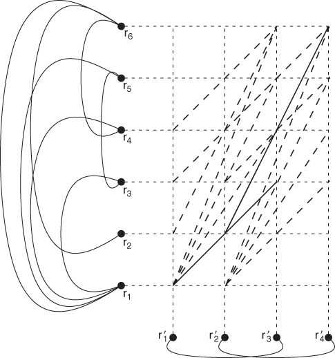
The reformulation hints at how DP can be used to solve the CMO problem. The central concept is to move from the lower left corner toward the upper right corner in an optimal fashion. Unlike the other alignment algorithms discussed in this section, which require a single application of DP, the method of A_purva requires a coupling of two DP algorithms. The two decisions are (1) where to link any possible match, called the local problem; and (2) how to construct on optimal sequence from the local decisions, called the global problem. The example in Figure 13.12 illustrates the decisions. From the match ![]() we could have selected any of
we could have selected any of ![]() ,
, ![]() ,
, ![]() or
or ![]() . In all but
. In all but ![]() we could have found a second nonintersecting edge that would have given a CMO score of 2. For example, if we had instead used the edge from
we could have found a second nonintersecting edge that would have given a CMO score of 2. For example, if we had instead used the edge from ![]() to
to ![]() , then we could have added the edge from
, then we could have added the edge from ![]() to
to ![]() . The local decision has to assess which edges should be considered. Once we know the optimal local solutions for each
. The local decision has to assess which edges should be considered. Once we know the optimal local solutions for each ![]() , we use this information to select the global collection of edges so as to maximize the number of edges while maintaining that edges don't cross.
, we use this information to select the global collection of edges so as to maximize the number of edges while maintaining that edges don't cross.
The forward-looking perspective means that we are always making decisions for indices in ![]() , and hence we need to account for the constraints whose summands are over
, and hence we need to account for the constraints whose summands are over ![]() . Andonov et al. [1] use a classic Lagrangian relaxation that moves these constraints to the objective and penalizes them with multipliers. The relaxed problem maximizes
. Andonov et al. [1] use a classic Lagrangian relaxation that moves these constraints to the objective and penalizes them with multipliers. The relaxed problem maximizes

subject to
We note that this is not directly a Lagrangian relaxation of (13.3) because of a tighter description of the feasible region. Specifically, the authors make the following replacements in (13.3):
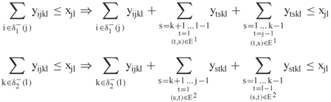
The additional terms continue to satisfy the noncrossing property, but they give a more accurate description of the search space.
The Lagrange multipliers ![]() and
and ![]() are restricted to be nonnegative, and through the application of DP, the relaxed problem can be solved in polynomial time for any collection of Lagrange multipliers, as the complexity is no worse than
are restricted to be nonnegative, and through the application of DP, the relaxed problem can be solved in polynomial time for any collection of Lagrange multipliers, as the complexity is no worse than ![]() . The local use of DP creates a scoring matrix for each
. The local use of DP creates a scoring matrix for each ![]() in
in ![]() . Specifically, let
. Specifically, let ![]() be the matrix whose rows are indexed by
be the matrix whose rows are indexed by ![]() and whose columns are indexed by
and whose columns are indexed by ![]() . The score at each position is
. The score at each position is ![]() , which corresponds to the coefficient of the
, which corresponds to the coefficient of the ![]() variable in the objective. Let
variable in the objective. Let ![]() be the optimal value of applying DP to
be the optimal value of applying DP to ![]() .
.
The global problem uses the local scores to create an optimal solution to the relaxed problem. Specifically, let ![]() be the scoring matrix whose components for each
be the scoring matrix whose components for each ![]() and
and ![]() are
are
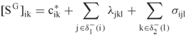
Note that the last two summations are the coefficients for the ![]() variables, and that the remaining portion of the objective collapses into
variables, and that the remaining portion of the objective collapses into ![]() . Hence, an optimal solution to the Lagrangian relaxation for any nonnegative collections of
. Hence, an optimal solution to the Lagrangian relaxation for any nonnegative collections of ![]() and
and ![]() can be calculated with a double application of DP.
can be calculated with a double application of DP.
While the relaxation can be solved efficiently, the relaxed solution is not a solution to the original CMO problem unless the Lagrange multipliers satisfy an optimality condition of their own. The optimization problem that defines a collection of multipliers for which the relaxed problem actually solves the CMO problem is called the dual-optimization problem, which is a minimization problem over the Lagrange multipliers for a fixed collection of ![]() and
and ![]() variables. A discussion of this topic is outside the scope of this chapter, but interested readers can find descriptions in most nonlinear programming texts [2]. The Lagrangian process is iterative in that starting with initial Lagrange multipliers, the relaxation is solved with DP, and then the Lagrange multipliers are updated by (nearly) solving the dual problem. The process repeats and is stopped once the value of the CMO problem is sufficiently close to the optimal value of the dual problem or due to a time limitation. For details about how A_purva updates the Lagrange multipliers, see the paper by Andonov et al. [1].
variables. A discussion of this topic is outside the scope of this chapter, but interested readers can find descriptions in most nonlinear programming texts [2]. The Lagrangian process is iterative in that starting with initial Lagrange multipliers, the relaxation is solved with DP, and then the Lagrange multipliers are updated by (nearly) solving the dual problem. The process repeats and is stopped once the value of the CMO problem is sufficiently close to the optimal value of the dual problem or due to a time limitation. For details about how A_purva updates the Lagrange multipliers, see the paper by Andonov et al. [1].
Iterative Lagrangian algorithms are a mainstay in the nonlinear programming community, and a common sentiment among experts in optimization is that problems either do or do not lend themselves to this tactic. The numerical tests for A_purva show that the relaxation of CMO lends itself nicely to this solution procedure. A_purva was tested as a database comparison algorithm on both Skolnick40 [6] and Proteus300 [1]. Reported solution times were ![]() s for all
s for all ![]() pairwise comparisons for Skolnick40 (approximately
pairwise comparisons for Skolnick40 (approximately ![]() s per comparison) and 13 h and 38 min for all 44,850 comparisons for Proteus300 (approximately 1.09 s per comparison). The comparisons were perfect in their agreement with the SCOP classification via clustering with Chavl [16]. Although not as fast as either of the other techniques discussed in this section, the results are significant advances for CMO, which before A_purva would have been impractical for a dataset like Proteus300.
s per comparison) and 13 h and 38 min for all 44,850 comparisons for Proteus300 (approximately 1.09 s per comparison). The comparisons were perfect in their agreement with the SCOP classification via clustering with Chavl [16]. Although not as fast as either of the other techniques discussed in this section, the results are significant advances for CMO, which before A_purva would have been impractical for a dataset like Proteus300.
13.4.4 Comments on Dynamic Programming and Future Research Directions
The application of DP to align protein structures is not restricted to the more recent literature on database applications, and in particular, DP was one of the early solution methods for the CMO problem, [6, 14]. However, the more recent literature indicates that DP is becoming a central algorithmic method to efficiently align protein structures well enough for classification across a sizable database. Other research groups are arriving at the same conclusion about DP [24]. Indeed, as the authors were preparing this document they found additional examples in the more recent literature [5].
With the emerging success that DP is having, we feel compelled to note a few of its limitations. First, DP is a sequential decision process that is optimal only under the Markov property, that is, that the current decision does not depend on past decisions. All the applications of DP discussed here use the natural sequence of the backbone to order the decisions process, but using DP in this fashion does not allow for the possibility of nonsequential alignments. The ability to identify nonsequential alignments is argued by some as a crucial element to identifying protein families [8]. Adapting the DP framework to consider nonsequential alignments is a promising and important avenue for future research.
One of the concerns about three-dimensional alignment methods is that they don't easily adapt to a protein's natural flexibility. Many proteins have several confirmations, and an alignment method that can correctly classify the different confirmations would be beneficial. Moreover, the crystallography and NMR experiments from which we gain three-dimensional coordinates are not without error, and the alignment methods should be robust enough to correctly classify proteins under coordinate perturbations. Whether methods based on DP provide the robustness to handle a protein's flexibility and experimental error is not yet well established. Hasegawa and Holm [10] suggest that more attention should be focused on the robustness of the optimization procedures used to align protein structures.
Finally, DP requires tuning that is experimental in nature. The gap opening and gap extension penalties need to be experimentally set to achieve agreement with biological classifications. Parameter tuning has not been shown to be database-independent, and without such experimental validation, we lack the confidence that DP-based methods can be used to organize a database without an a priori biological classification, which somewhat defeats the purpose of automating database classification.
References
1. Andonov R, Malod-Dognin N, Yanev N, Maximum contact map overlap revisited, J. Comput. Biol. 18(1):27–41 (Jan. 2011).
2. Bazaraa M, Sherali H, Shetty C, Nonlinear Programming: Theory and Algorithms, 3rd ed., Wiley-Interscience, 2006.
3. Bellman R, Dynamic Programming, Princeton Univ. Press, Princeton, NJ, 1957.
4. Bhattacharya S, Bhattacharyya C, Chandra N, Projections for fast protein structure retrieval, BMC Bioinformatics 7(Suppl. 5):S5 (2006).
5. Bonnel N, Marteau P, LNA: Fast Protein Classification Using a Laplacian Characterization of Tertiary Structure, Technical Report, Univ. Bretagne Sud, France, 2011.
6. Caprara A, Carr R, Istrail S, Lancia G, Walenz B, 1001 optimal pdb structure alignments: Integer programming methods for finding the maximum contact map overlap, J. Comput. Biol. 11(1):27–52 (2004).
7. Carpentier M, Brouillet S, Pothier J, Yakusa: A fast structural database scanning method, Proteins 61(1):137–151 (Oct. 2005).
8. Chen L, Wu L, Wang Y, Zhang S, Zhang X, Revealing divergent evolution, identifying circular permutations and detecting active-sites by protein structure comparison, BMC Struct Biol. 6:18 (2006).
9. Goldman D, Istrail S, Papadimitriou C, Algorithmic aspects of protein structure similarity. Proc. 40th Annual Symp. Foundations of Computer Science, 1999, pp. 512–521.
10. Hasegawa H, Holm L, Advances and pitfalls of protein structural alignment, Curr. Opin. Struct. Biol. 19(3):341–348 (June 2009).
11. Holder A, Simon J, Strauser J, Shibberu Y, An Investigation into the Robustness of Algorithms Designed for Efficient Protein Structure Alignment across Databases, Technical Report, Rose-Hulman Inst. Technology, 2012.
12. Kifer I, Nussinov R, Wolfson H, Gossip: A method for fast and accurate global alignment of protein structures, Bioinformatics 27(7):925–932 (2011).
13. Kolodny R, Linial N, Approximate protein structural alignment in polynomial time, Proc Natl Acad Sci USA 101(33):12201–12206 (Aug. 2004).
14. Lancia G, Carr R, Walenz B, Istrail S, 101 optimal pdb structure alignments: A branch-and-cut algorithm for the maximum contact map overlap problem, Proc. 5th Annual Int. Conf. Computational Biology, ACM Press, New York, 2001, pp. 143–202.
15. Di Lena P, Fariselli P, Margara L, Vassura M, Casadio R, Fast overlapping of protein contact maps by alignment of eigenvectors, Bioinformatics 26(18):2250–2258 (Sept. 2010).
16. Lerman I, Likelihood linkage analysis (lla) classification method, Biochimie 75:379–397 (1993).
17. Cheng Li S, Kaow Ng Y, On protein structure alignment under distance constraint, Theor. Comput. Sci. 412(32):4187–4199 (2011) (algorithms and computation).
18. Needleman S, Wunsch C, A general method applicable to the search for similarities in the amino acid sequence of two proteins, J. Mol. Biol. 48(3):443–453 (March 1970).
19. Poleksic A, Algorithms for optimal protein structure alignment, Bioinformatics, 25(21):2751–2756 (Nov. 2009).
20. Poleksic A, Optimizing a widely used protein structure alignment measure in expected polynomial time, IEEE/ACM Trans. Comput. Biol. Bioinform. 8(6):1716–1720 (2011).
21. Shatsky M, Nussinov R, Wolfson H, A method for simultaneous alignment of multiple protein structures, Proteins 56(1):143–156 (July 2004).
22. Shibberu Y, Holder A, A spectral approach to protein structure alignment, IEEE/ACM Trans. Comput. Biol. Bioinform. 8:867–875 (Feb. 2011).
23. Umeyama S, An eigendecomposition approach to weighted graph matching problems, IEEE Trans. Pattern Anal. Machine Intell. 10(5):695–703 (1988).
24. Wohlers I, Andonov R, Klau G, Algorithm Engineering for Optimal Alignment of Protein Structure Distance Matrices, Technical Report, CWI, Life Sciences Group, Netherlands, 2011.
25. Xu J, Jiao F, Berger B, A parameterized algorithm for protein structure alignment, J. Comput. Biol. 14(5):564–577 (June 2007).