
Chapter 12
Computational Methods in CryoElectron Microscopy 3D Structure Reconstruction
12.1 Introduction
Electron cryomicroscopy (cryoEM) is a rapidly emerging tool in structural biology for three-dimensional (3D) structure determination of macromolecular complexes. Single-particle cryoEM allows structural elucidation of macromolecular assemblies at subnanometer resolution [1, 2], and, in some cases, at atomic resolution [3]. Electron cryotomography (ET) allows structural studies of complex speciments at near-molecular resolution as well as visualization of macromolecular complexes in their native cellular context [4]. The integrative combination of these cryoEM modalities with other high-resolution approaches, such as X-ray crystallography or nuclear magnetic resonance (NMR), is expected to provide a comprehensive description of the cellular function in molecular detail [5].
In ET, a series of projection images where structural features from different layers of the 3D structure of the specimen are first superposed along the direction of the electron beam. In general, those images are obtained by tilting the specimen around tilt axes [6]. The 3D structure of the sample can then be derived from those projection images, by means of tomographic reconstruction algorithms [7]. Because of physical limitations of microscopes, the angular tilt range is limited and, as a result, tomographic tilt series have a wedge of missing data corresponding to the uncovered angular range. Moreover, biological material is very sensitive to radiation, so specimens must be imaged at very low electron doses, which makes projection images extremely noisy. In high-resolution structural studies, this poor signal-to-noise ratio (SNR) is in the order of only 0.1 [8]. As a consequence, high-resolution electron tomography requires a method of 3D reconstruction from projections able to deal with limited angle conditions and extremely low SNR of the projection images.
In terms of computation, there are several main problems in ET reconstruction: the extremely low SNR of the images, alignment and classification of the images, 3D reconstruction under limited angle conditions, and post-processing and interpretation of the reconstruction results [8]. Also, because of the poor SNR in projection images, the size of tomograms and the number of projectionimages increase for high-resolution studies, and the computation time for 3D reconstruction also increases, which becomes a bottleneck for routine applicaitons of ET.
Since the demands of huge computational costs and resources derive from the computational complexity of the recontruction algorithms and the large size and number of the projection images involved, this chapter addresses the 3D reconstruction algorithm and its multilevel parallel strategy on GPU platform. We present an adaptive simulatneous algebraic reconstruction technique (ASART) for imcomplete data and noisy conditons. Specifically, we develop three key techniques—modified multilevel access scheme (MMAS), adaptive adjustment of relaxation (AAR) parameters, and column sum substitution (CSS) technique, to improve the reconstruction quality and speed of the reconstruction process. Also, we present a multilevel parallel strategy for iterative reconstruction algorithm in ET on multi-GPUs, and we develop an asynchronous comunication scheme and data structure named blob-ELLR to accelerate reconstruction processing and reduce memory requirements.
The remainder of the chapter is organized as follows Section 12.2 reviews icterative 3D reconstruciton methods for ET. Section 12.3 focuses on the ASART algorithm. Section 12.4 presents a multilevel parallel strategy for iterative reconstruction algorithm. Section 12.5 shows and analyzes the experimental results. Section 12.6 concludes the chapter with a summary.
12.2 Iterative image reconstruction methods
In ET, the projection images are acquired from a specimen through so-called single-axis tilt geometry. The specimen is tilted over a range, typically from −60° (or −70°) to +60° (or +70°) due to physical limitations of microscopes, with small tilt increments (1° or 2°). An image of the same object area is recorded at each tilt angle, and then the 3D reconstruction of the specimen can be obtained from a set of projection images by reconstruction methods.
Several reconstruction methods for ET have been proposed. Weighted backprojection (WBP) has been one of the most popular methods in the field of 3D reconstruction of ET, due to its algorithmic simplicity and computational efficiency [9]. The major disadvantage of WBP, however, is that the results may be strongly affected by limited-angle data and noisy conditions [10]. Series expansion methods (i.e., iterative methods) constitute one of the main alternatives to WBP in 3D reconstruction of ET, owing to their good performance in handling incomplete and noisy data. Several traditional iterative methods, such as algebraic reconstruction techniques (ARTs) [11, 12], simultaneous iterative reconstruction technique(SIRT) [13], component averaging methods (CAVs) [10], block-iterative CAV (BICAV) [10], and simultaneous algebraic reconstruction technique (SART) [14] have all been utilized to 3D reconstruction of ET. ART enjoys a rapid convergence but exhibits a very noisy salt-and-pepper image characteristic of reconstructed images. SIRT and CAV, on the contrary, produce fairly smooth reconstructed images, but still require a large number of iterations for convergence. SART is characterized by better robustness than ART under noise, and its convergence speed is reported to be faster than that of SIRT and CAV [14].
In this section, we give a brief overview of blob-based iterative reconstruction methods and describe the simultaneous algebraic reconstruction technique (SART).
12.2.1 Blob-Based Iterative Reconstruction Methods
Iterative methods are based on the series expansion approach [15], in which 3D volume ![]() is represented as a linear combination of a limited set of known and fixed basis functions
is represented as a linear combination of a limited set of known and fixed basis functions ![]() , with appropriate coefficients
, with appropriate coefficients ![]() , that is
, that is
12.1 
where (![]() ) is a spherical coordinate, and
) is a spherical coordinate, and ![]() is the total number of the unknown variables
is the total number of the unknown variables ![]() . In 3D reconstruction, the basis functions used to represent the object greatly influences the reconstructed results. During the 1990s, spherically symmetric volume elements (called blobs) were thoroughly investigated and, as a consequence, the conclusion that blobs yield better reconstructions than the traditional voxels has been drawn in 3D reconstruction [16]. The use of blob basis functions provides iterative methods with better resolution–noise performance than voxel basis functions because of the overlapping nature of their rotational symmetric basis functions. Thus, we consider the blob basis instead of the traditional voxel one. The blob basis discussed in this chapter is constructed using generalized Kaiser–Bessel (KB) window functions
. In 3D reconstruction, the basis functions used to represent the object greatly influences the reconstructed results. During the 1990s, spherically symmetric volume elements (called blobs) were thoroughly investigated and, as a consequence, the conclusion that blobs yield better reconstructions than the traditional voxels has been drawn in 3D reconstruction [16]. The use of blob basis functions provides iterative methods with better resolution–noise performance than voxel basis functions because of the overlapping nature of their rotational symmetric basis functions. Thus, we consider the blob basis instead of the traditional voxel one. The blob basis discussed in this chapter is constructed using generalized Kaiser–Bessel (KB) window functions
12.2 
where ![]() (
(![]() ) denotes the modified Bessel function of the first kind of order m, a is the radius of the blob, and
) denotes the modified Bessel function of the first kind of order m, a is the radius of the blob, and ![]() is a nonnegative real number controlling the shape of the blob. The choice of the parameters
is a nonnegative real number controlling the shape of the blob. The choice of the parameters ![]() , and
, and ![]() will influence the quality of blob-based reconstructions. The basis functions that developed by Matej and Lewitt are used for the choice of the parameters in our algorithm (i.e.,
will influence the quality of blob-based reconstructions. The basis functions that developed by Matej and Lewitt are used for the choice of the parameters in our algorithm (i.e., ![]() ,
, ![]() ,
, ![]() ).
).
In 3D ET, the model of the image formation process is expressed by the following linear system
where ![]() denotes the
denotes the ![]() th measured image of
th measured image of ![]() is the dimension of
is the dimension of ![]() , where
, where ![]() is the number of projection angles and
is the number of projection angles and ![]() the number of projection values per view; and
the number of projection values per view; and ![]() is a weighting factor representing the contribution of the
is a weighting factor representing the contribution of the ![]() th basis function to the
th basis function to the ![]() th projection. Under such a model, the element
th projection. Under such a model, the element ![]() can be calculated according to the projected procedure as follows:
can be calculated according to the projected procedure as follows:
12.4 ![]()
12.5 ![]()
where ![]() is the projected value of the pixel
is the projected value of the pixel ![]() at an angle
at an angle ![]() ;
; ![]() is defined as a sparse matrix with
is defined as a sparse matrix with ![]() rows and
rows and ![]() columns where
columns where ![]() is the element of
is the element of ![]() . In general, the storage demand of the weighted matrix
. In general, the storage demand of the weighted matrix ![]() rapidly increases as the size and number of projection images increase. For example, when the size of images is
rapidly increases as the size and number of projection images increase. For example, when the size of images is ![]() , the storage demand of the matrix approaches 3.5 GB.
, the storage demand of the matrix approaches 3.5 GB.
Under those assumptions, the image reconstruction problem can be modeled as the inverse problem of estimating the ![]() values from the
values from the ![]() values by solving the system of linear equations given byEquation (12.3). This problem is usually resolved by means of iterative methods.
values by solving the system of linear equations given byEquation (12.3). This problem is usually resolved by means of iterative methods.
12.2.2 Simultaneous Algebraic Reconstruction Technique (SART)
The SART algorithm is a basic iterative method designed to solve the linear system in image reconstruction. Typically, the algorithm begins with an arbitrary ![]() and then begins to iterate until convergence [18]. The arbitrary initial value may greatly deviate from the true value. So the number of iterations can be very large. In order to accelerate the process of convergence, SART further adopts a backprojection technique (BPT), a simple WBP without the weighting functions, to estimate the first approximation
and then begins to iterate until convergence [18]. The arbitrary initial value may greatly deviate from the true value. So the number of iterations can be very large. In order to accelerate the process of convergence, SART further adopts a backprojection technique (BPT), a simple WBP without the weighting functions, to estimate the first approximation ![]() [19]. BPT is a simple reconstruction method where the gray level of a pixel can be considered as the weighted average of the projections for all the possible rays passing through the pixel [7, 20]. Consequently, the initial solution
[19]. BPT is a simple reconstruction method where the gray level of a pixel can be considered as the weighted average of the projections for all the possible rays passing through the pixel [7, 20]. Consequently, the initial solution ![]() is defined by as follows:
is defined by as follows:
12.6 
Then, in an iterative process, SART is described by the following expression
12.8 
where ![]() is the number of iterations,
is the number of iterations, ![]() is the relaxation parameter,
is the relaxation parameter, ![]() is the fixed value (in general, 0 <
is the fixed value (in general, 0 < ![]() < 2),
< 2), ![]() is the number of projections per view, and
is the number of projections per view, and ![]() =
= ![]() +
+ ![]() denotes the
denotes the ![]() th equation of the system;
th equation of the system; ![]() is the number of all views obtained
is the number of all views obtained ![]() = (
= (![]() is the index of the view, and
is the index of the view, and ![]() is the next iterative value obtained by updating
is the next iterative value obtained by updating ![]() . SART adopts a view-by-view strategy; that is, an approximation is updated simultaneously by all the projections of each view.
. SART adopts a view-by-view strategy; that is, an approximation is updated simultaneously by all the projections of each view.
As mentioned above, the convergence speed of SART is higher than that of SIRT and CAV; the convergence process of SART is still slow and it is difficult to acquire satisfactory results:
12.3 Adaptive simultaneous algebraic reconstruction technique (ASART)
To generate high-quality reconstructions with improved computational speed, we have developed a technique known more popularly by its acronym, ASART. The key techniques developed in ASART include a modified multilevel access scheme (MMAS) to arrange the order of projection data, an adaptive adjustment of relaxation parameters (AAR) to correct the discrepancy between actual and computed projections, and a column sum substitution (CSS) to reduce the memory requirement and computation time.
12.3.1 Modified Multilevel Access Scheme (MMAS)
The SART method adopts SAS to order the views so that there is a high correlation between consecutive views. The convergence can be significantly facilitated if the views are ordered to maximize their orthogonality [21]. Toward this goal, a multilevel access scheme (MAS) is adopted to substantially decrease the correlated error between the consecutive views. A detailed comparison between MAS and SAS shows that MAS yields the most efficient reconstruction [26]. Applications in different situations have shown that MAS can obtain promising results [27, 28].
The MAS method is based on the fact that two views of ![]() apart are minimally correlated, and the third view is set to the angle halving the former two views to minimize the correlation of three views [21]. The MAS ordering applies to any number of views but works best if the number of views is a power of 2. Suppose that the views are indexed as 0, 1, …,
apart are minimally correlated, and the third view is set to the angle halving the former two views to minimize the correlation of three views [21]. The MAS ordering applies to any number of views but works best if the number of views is a power of 2. Suppose that the views are indexed as 0, 1, …, ![]() , where
, where ![]() is the number of views. In MAS, views can be organized in a total of
is the number of views. In MAS, views can be organized in a total of ![]() levels where
levels where ![]() is expressed by
is expressed by
12.9 ![]()
In level ![]() , view 0 (
, view 0 (![]() ) and view
) and view ![]() /2 (90
/2 (90![]() ) with a maximum orthogonality are accessed first. Then, in level
) with a maximum orthogonality are accessed first. Then, in level ![]() , there are two views: 45
, there are two views: 45![]() and 135
and 135![]() (or whose indices are
(or whose indices are ![]() /4 and
/4 and ![]() /4). Furthermore, in level
/4). Furthermore, in level ![]() , the indices of views are respectively
, the indices of views are respectively ![]() /8,
/8, ![]() /8,
/8, ![]() /8, and
/8, and ![]() /8. In every level, the views with the odd indices and the following ones with even indices are orthogonal.
/8. In every level, the views with the odd indices and the following ones with even indices are orthogonal.
As described above, MAS is adapted for the complete projection views distributed uniformly from 0![]() to 180
to 180![]() . However, the projection views of ET are incomplete and limited in a certain range. We cannot always find two projections whose views are 90
. However, the projection views of ET are incomplete and limited in a certain range. We cannot always find two projections whose views are 90![]() apart. If MAS is directly used to arrange the order of the views in ET, some views to which there are no views perpendicular will be left. If these views that remain unprocessed by MAS are then arranged by SAS, there will be a high correlation between the consecutive views. We propose a modified MAS (MMAS) to arrange the order of projections in ASART. Only a series of projections evenly distributed across the whole angle is considered as ET projections. For example, the tilt angle ranges from
apart. If MAS is directly used to arrange the order of the views in ET, some views to which there are no views perpendicular will be left. If these views that remain unprocessed by MAS are then arranged by SAS, there will be a high correlation between the consecutive views. We propose a modified MAS (MMAS) to arrange the order of projections in ASART. Only a series of projections evenly distributed across the whole angle is considered as ET projections. For example, the tilt angle ranges from ![]() to +60
to +60![]() with a small tilt increment of 2
with a small tilt increment of 2![]() . In MMAS, we adopt the range
. In MMAS, we adopt the range ![]() (
(![]() ) of tilt angles as the selected factor instead of
) of tilt angles as the selected factor instead of ![]() since the range is 120
since the range is 120![]() rather than 180
rather than 180![]() . Note that the range for the tilt angles can still vary in different situations. In the first level, we choose view
. Note that the range for the tilt angles can still vary in different situations. In the first level, we choose view ![]() and view 0
and view 0![]() between whom the angle is the half of the range (but not 90
between whom the angle is the half of the range (but not 90![]() ). The two views that halve the angles between the first two are in the second level (i.e., view
). The two views that halve the angles between the first two are in the second level (i.e., view ![]() and view 30
and view 30![]() ). In such a scheme,views in one level will halve (or almost) the views in all previous levels. Figure 12.1 shows the situation for the example by labeling the order of access in our MMAS scheme on the corresponding view angles. The proposed scheme clearly covers all angular regions evenly over time as shown in Figure 12.1. Table 12.1 summarizes the results of every level for this example. Note that in any level, the computed value of views may not be included in the projected views or may have already been accessed. If so, we search both sides of the computed value until the closest unused value is found and then put it into the sequence. Before the iterative process of ASART is carried out, the order of the overall views is arranged according to MMAS as discussed above.
). In such a scheme,views in one level will halve (or almost) the views in all previous levels. Figure 12.1 shows the situation for the example by labeling the order of access in our MMAS scheme on the corresponding view angles. The proposed scheme clearly covers all angular regions evenly over time as shown in Figure 12.1. Table 12.1 summarizes the results of every level for this example. Note that in any level, the computed value of views may not be included in the projected views or may have already been accessed. If so, we search both sides of the computed value until the closest unused value is found and then put it into the sequence. Before the iterative process of ASART is carried out, the order of the overall views is arranged according to MMAS as discussed above.
Figure 12.1 The access orders of the first three levels for the example. The left bold numbers on the left denote the index of access, and ![]() denotes the number of the level.
denotes the number of the level.
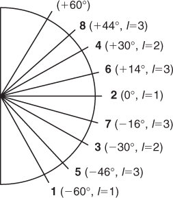
Table 12.1 Access Orders for ![]() Projections Ranging from
Projections Ranging from ![]() to +60
to +60![]() (
(![]() )
)
12.3.2 Adaptive Adjustment of Relaxation Parameters (AARPs)
In SART, the gray level ![]() is corrected by the relaxation parameters
is corrected by the relaxation parameters ![]() and the discrepancies between the actual projections
and the discrepancies between the actual projections ![]() and the computed projections
and the computed projections ![]() in each iteration. As shown in Equation (12.7 ), the relaxation parameters
in each iteration. As shown in Equation (12.7 ), the relaxation parameters ![]() are determined only by the weight
are determined only by the weight ![]() and the fixed value
and the fixed value ![]() in the iterative procedure. The convergence process can be faster if the relaxation parameters are adjusted as a function of the number of iterations. The relaxation parameters are determined in such a way that they decrease as the number of iterations increases [19]. In SART, the relaxation parameters are determined only by the weight
in the iterative procedure. The convergence process can be faster if the relaxation parameters are adjusted as a function of the number of iterations. The relaxation parameters are determined in such a way that they decrease as the number of iterations increases [19]. In SART, the relaxation parameters are determined only by the weight ![]() while the gray level
while the gray level ![]() is ignored. Thus the pixels with large gray levels will have the same backprojection of the discrepancies as the pixels with small gray levels.
is ignored. Thus the pixels with large gray levels will have the same backprojection of the discrepancies as the pixels with small gray levels.
In fact, the pixels with different gray levels make different contributions to the discrepancies. In ASART, a data-driven adjustment of relaxation parameters (AAR) is applied during the reconstruction procedure. In AAR, the relaxation parameters are determined according to the gray levels as well as the weights as shown in the following equation:
With this approach, the relaxation parameter for each pixel is adjusted according to its gray level obtained in the previous iteration. Note that ![]() represents the geometry contribution of the
represents the geometry contribution of the ![]() pixel only to the
pixel only to the ![]() ray integral. According to Eq. (12.10), the contribution of the
ray integral. According to Eq. (12.10), the contribution of the ![]() pixel to the
pixel to the ![]() ray integral includes both the geometry contribution
ray integral includes both the geometry contribution ![]() and the contribution of the gray level
and the contribution of the gray level ![]() of the
of the ![]() pixel. This is different from SART, where the gray level
pixel. This is different from SART, where the gray level ![]() of the
of the ![]() pixel is not considered as shown in Equation (12.7).
pixel is not considered as shown in Equation (12.7).
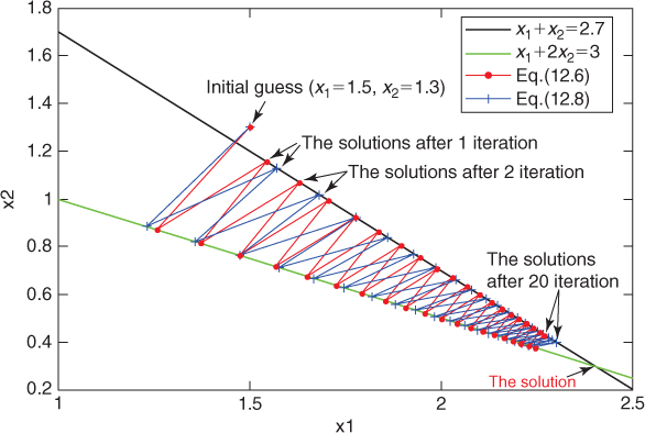
To illustrate intuitively how the convergence process can be accelerated by AAR, we consider a case with only two variables ![]() and
and ![]() satisfying the following equations:
satisfying the following equations:
12.11 
The computational procedures for locating the solution from an initial guess (![]() =1.5,
=1.5, ![]() =1.3) are displayed in Figure 12.2. The line in red denotes the procedure with the constant relaxation parameter by Eq. (12.7), and the line in blue describes the process with the adaptive relaxation parameter by Eq. (12.10). It is seen that the solution obtained by Eq. (12.10) is closer to the true solution than that obtained by Eq. (12.7) after the same number of iterations.
=1.3) are displayed in Figure 12.2. The line in red denotes the procedure with the constant relaxation parameter by Eq. (12.7), and the line in blue describes the process with the adaptive relaxation parameter by Eq. (12.10). It is seen that the solution obtained by Eq. (12.10) is closer to the true solution than that obtained by Eq. (12.7) after the same number of iterations.
Figure 12.2 Illustration of the computational procedures from an initial guess.
Note that in fact we don't need to recompute the sum of ![]() in Eq. (12.10) since it is equal to
in Eq. (12.10) since it is equal to ![]() , which has been computed in the process of reprojection. Extra computation is needed only for the multiplication of
, which has been computed in the process of reprojection. Extra computation is needed only for the multiplication of ![]() and
and ![]() , but it is not time-consuming compared with the total computation.
, but it is not time-consuming compared with the total computation.
12.3.3 Column Sum Substitution Technique (CSS)
We define ![]() as the reciprocal of the sum of the
as the reciprocal of the sum of the ![]() th column in each view by
th column in each view by
12.12 ![]()
Although the column sums remain unchanged in each iteration, large memory space is needed to store each column sum for a SART reconstruction of large images. In fact, it has been proved that ![]() has no effect on the final solution to which SART converges [29]. In another iterative method called BICAV (block-iterative component averaging) [10], the relaxation parameters are generated by the following equation
has no effect on the final solution to which SART converges [29]. In another iterative method called BICAV (block-iterative component averaging) [10], the relaxation parameters are generated by the following equation
12.13 ![]()
where ![]() denotes the number of times that components
denotes the number of times that components ![]() of the volume contributes with nonzero value to the equations in the
of the volume contributes with nonzero value to the equations in the ![]() th block. This is called oblique projection in BICAV. SART, on the other hand, is based on orthogonal projections. It has been proved that oblique projections allow iterative methods to have higher convergence speeds, especially during the early stages of iterations [10].
th block. This is called oblique projection in BICAV. SART, on the other hand, is based on orthogonal projections. It has been proved that oblique projections allow iterative methods to have higher convergence speeds, especially during the early stages of iterations [10].
Accordingly, we propose that ![]() is replaced by a scalar
is replaced by a scalar ![]() denoting the maximum number of the nonzero weight
denoting the maximum number of the nonzero weight ![]() in each view. In this way, the memory requirement and computation time are reduced, and the high qualities of the results are obtained because of this oblique projections. In the blob (if the radius
in each view. In this way, the memory requirement and computation time are reduced, and the high qualities of the results are obtained because of this oblique projections. In the blob (if the radius ![]() =2), the maximum number of the rays that affect every pixel on its reconstructed gray level in each view is 4. The relaxation parameter
=2), the maximum number of the rays that affect every pixel on its reconstructed gray level in each view is 4. The relaxation parameter ![]() with our CSS technique can be expressed by
with our CSS technique can be expressed by
12.14 
This modification can conserve runtime because the algorithm doesn't need to compute each column sum ![]() for each view. The modification can also reduce the memory requirement by using the scalar
for each view. The modification can also reduce the memory requirement by using the scalar ![]() instead of the vector
instead of the vector ![]() , especially when the size of the image is very large.
, especially when the size of the image is very large.
With the improvements mentioned above, ASART is formulated as follows:
12.15 
12.4 Multilevel parallel strategy for iterative reconstruction algorithm
The reconstruction time of blob-based iterative methods is a major challenge in ET because of the large reconstructed data volume. So parallel computing on multiple GPUs is becoming paramount to satisfying the computational requirement. In this section, we present a multilevel parallel strategy for blob-based iterative reconstruction and implement it on the OpenMP-CUDA architecture.
12.4.1 Coarse-Grained Parallel Scheme Using OpenMP
In the first level of the multilevel parallel scheme, a coarse-grained parallelization is straightforward in line with the properties of ET reconstruction. The single-tilt axis geometry allows data decomposition into slabs of slices orthogonal to the tilt axis. For this decomposition, the number of slabs equals the number of GPUs, and each GPU reconstructs its own slab. Consequently, the 3D reconstruction problem can be decomposed into a set of 3D slab reconstruction subproblems. However, the slabs are interdependent because of the overlapping nature of blobs. Therefore, each GPU has to receive a slab that is composed of its corresponding own slices and additional redundant slices reconstructed in neighbor slabs. The number of redundant slices depends on the blob extension. In a slab, its own slices are reconstructed by the corresponding GPU and require information provided by the redundant slices from the neighbor GPUs. During the process of 3DET reconstruction, each GPU has to communicate with other GPUs for the additional redundant slices.
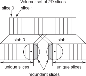
We have implemented the 3DET reconstruction based on the architecture in which a CPU controls several GPUs and the GPUs share the memory. We adopt two GPUs in the different platforms to implement the blob-based reconstruction. Thus the first-level parallel strategy makes use of two GPUs to perform the coarse-grained parallelization of the reconstruction. As shown in Figure 12.3, the 3D volume data are halved into two slabs, and each slab contains its own slices and a redundant slice. According to the shape of the blob adopted (the blob radius is 2 in our experiments), only one redundant slice is included in each slab. Each slab is assigned to and reconstructed on each individual GPU in parallel. A shared-memory parallel programming scheme (OpenMP) is employed to fork two threads to control the separated GPU. Each slab is reconstructed on each individual GPU by each parallel thread. Consequently, the partial results attained by GPUs are combined to complete the final result of the 3D reconstruction. Certainly, the parallel strategy can be applied on GPU clusters. In a GPU cluster, the number of slabs equals the number of GPUs for the decomposition described above.
Figure 12.3 Coarse-grained parallel scheme using blob. 3D volume is decomposed into slabs of slices. The number of slabs equals the number of GPUs.
12.4.2 Fine-Grained Parallel Scheme Using CUDA
In the second level of the multilevel parallel scheme, 3D reconstruction of one slab, as a fine-grained parallelization, is implemented on each GPU using CUDA. In the 3D reconstruction of a slab, the generic iterative process is described as follows:
- Initiation—compute the wight matrix
 and create an initial value for
  by BPT.
 - Reprojection—estimate the computed projection data
 basis of the on the current approximation
  .
. - Comparison—compare and compute the discrepancy
 between the real experimental and calculated projections.
 - Backprojection—backproject the comparison results over the image space and obtain
 .
. - Refinement—update the current approximation
 by incorporating the weighted backprojection
  .
.
The interdependence among neighbor slabs implies that, after computation of either the reprojection or backprojection for a given slab, there must be a proper exchange of information between neighboring GPUs.
12.4.3 Asynchronous Communication Scheme
As described above for the multilevel parallel scheme, there must be two communications between neighbor GPUs during one iterative reconstruction process: (1) to exchange the computed projections of the redundant slices after the reprojection process and (2) to exchange the reconstructed pixels of the redundant slices after the backprojection process. CUDA provides a synchronous communication scheme [cudaThreadSynchronize(#)] to accommodate the communication between GPUs. With the synchronous communication scheme, GPUs must sit idle while data are exchanged, which has a negative impact on the performance of the reconstruction in ET.
In the 3DET reconstruction on clusters, the use of blobs as basis functions involves significant additional difficulties in the parallelization and necessitates substantial communications among the processors. In any parallelization project where communication between nodes is involved, latency hiding becomes an issue [30]. An effective strategy stands for overlapping communication and computing so as to keep the processor busy while waiting for the communications to be completed [10]. In this study, a latency hiding strategy has been devised to deal with the communications efficiently. To minimize the idle time on the GPUs, we also present a latency hiding strategy using an asynchronous communication scheme in which different streams are used to perform GPU execution and CPU-GPU memory access asynchronously. The communication scheme splits GPU execution and memory copies into separate streams. Execution in one stream can be performed at the same time as a memory copy from another. In one slab reconstruction, reprojection of the redundant slices, memory copies and backprojection of the redundant slices are performed in one stream. The executions (i.e., reprojection and backprojection) of the slab's own slices are performed in the other stream. This can be extremely useful for reducing the idle time of GPUs.
12.4.4 Blob-ELLR Format with Symmetric Optimization Techniques
In the parallel blob-based iterative reconstruction, another problem is the lack of memory on GPUs for the sparse weighted matrix. Several data structures have been developed to store sparse matrices. Compressed row storage (CRS) and ELLPACK are the most two extended formats to store the sparse matrix on CPUs [31]. ELLPACK-R (ELLR), a variant of the ELLPACK format, has been proved to outperform the most efficient formats for storing the sparse matrix data structure on GPUs. ELLR consists of two arrays, ![]() [#] and
[#] and ![]() [#] of dimension
[#] of dimension ![]() , and an additional
, and an additional ![]() -dimensional integer array called
-dimensional integer array called ![]() [#] is included in order to store the actual number of nonzeros in each row [33]. With the size and number of projection images increasing, the memory demand of the sparse weighted matrix rapidly increases. The weighted matrix involved is too large to load into most of GPUs because of the limited available memory, even with the ELLR data structure.
[#] is included in order to store the actual number of nonzeros in each row [33]. With the size and number of projection images increasing, the memory demand of the sparse weighted matrix rapidly increases. The weighted matrix involved is too large to load into most of GPUs because of the limited available memory, even with the ELLR data structure.
Vazquez et al. proposed a matrix approach and exploited several geometry-related symmetry relationships to reduce the weighted matrix involved in the WBP reconstruction method [32]. In our work, we present a data structure named blob-ELLR and exploit several geometric symmetry relationships to reduce the weighted matrix involved in iterative reconstruction methods. The blob-ELLR data structure decreases the memory requirement and then accelerates the speed of ET reconstruction on GPUs. Compared with the matrix approach [32], our matrix blob-ELLR is adopted to store the weighted matrix ![]() instead of the transpose of the one involved in the original ELLR. As shown in Figure 12.4 (a), the maximum number of rays related to each pixel is four because of the blob radius (viz.,
instead of the transpose of the one involved in the original ELLR. As shown in Figure 12.4 (a), the maximum number of rays related to each pixel is four because of the blob radius (viz., ![]() = 2). To store the matrix
= 2). To store the matrix ![]() , the blob-ELLR includes two 2D arrays: one float
, the blob-ELLR includes two 2D arrays: one float ![]() [#] to save the entries, and the other integer
[#] to save the entries, and the other integer ![]() [#] to save the columns of every entry (see Fig. 12.4b). Both arrays are of dimension
[#] to save the columns of every entry (see Fig. 12.4b). Both arrays are of dimension ![]() , where
, where ![]() is the number of columns of
is the number of columns of ![]() and
and ![]() is the maximum number of nonzeros in the columns (
is the maximum number of nonzeros in the columns (![]() is the number of the projection angles). Because the percentage of zeros is low in the blob-ELLR, it is not necessary to store the actual number of nonzeros in each column. Thus the additional integer array
is the number of the projection angles). Because the percentage of zeros is low in the blob-ELLR, it is not necessary to store the actual number of nonzeros in each column. Thus the additional integer array ![]() [#] is not included in the blob-ELLR.
[#] is not included in the blob-ELLR.
Figure 12.4 Blob-ELLR format with symmetric optimization techniques are exploited to reduce the storage space of ![]() to almost
to almost ![]() th of the original size.
th of the original size.

Although the blob-ELLR without symmetric techniques can reduce the storage of the sparse matrix ![]() , the number of
, the number of ![]() is rather large, especially when the number of
is rather large, especially when the number of ![]() increases rapidly. The optimization takes advantage of the symmetry relationships as follows:
increases rapidly. The optimization takes advantage of the symmetry relationships as follows:
12.16 ![]()
So, only ![]() need to be stored in the blob-ELLR, whereas the other elements are easily computed from
need to be stored in the blob-ELLR, whereas the other elements are easily computed from ![]() . This scheme can reduce the storage spaces of
. This scheme can reduce the storage spaces of ![]() and
and ![]() to 25%.
to 25%.
12.17 ![]()
It is easy to see that the point (![]() ) of a slice is then projected to a point
) of a slice is then projected to a point ![]() (
(![]() ) in the same tilt angle
) in the same tilt angle ![]() . The weighted value of the point (
. The weighted value of the point (![]() ) can be computed according to that of the point (
) can be computed according to that of the point (![]() ). Therefore, it is not necessary to store the weighted value of almost half of the points in the matrix
). Therefore, it is not necessary to store the weighted value of almost half of the points in the matrix ![]() so that the space requirements for
so that the space requirements for ![]() and
and ![]() are further reduced by nearly 50%.
are further reduced by nearly 50%.
With the three symmetric optimizations mentioned above, the size of the storage for two arrays in the blob-ELLR is almost ![]() reducing to nearly
reducing to nearly ![]() of the original size.
of the original size.
12.5 Experimental results and discussion
The objective of this study is to improve the quality and efficiency of 3D ET reconstruction. In this chapter, a reconstruction method ASART and a multilevel parallel strategy are presented. Two experiments have been carried out to evaluate the proposed methods, respectively. To evaluate the performance of ASART, we compare the reconstruction qualities of ASART with those of WBP and SART. To evaluate the performance of the multilevel parallel strategy, two different experimental datasets are reconstructed on Fermi platforms.
12.5.1 Materials and Computing Resources
All the experimental data in our work are the caveolae from the procine aorta endothelial (PAE) cell, collected by FEI Tecnai 20 in China National Key Laboratory of Biomacromolecules [34]. Two different experimental datasetsare used (denoted by small-sized and large-sized) with 112 images of ![]() pixels, and 119 images of
pixels, and 119 images of ![]() pixels, to reconstruct tomograms of
pixels, to reconstruct tomograms of ![]() and
and ![]() , respectively.
, respectively.
The first experiment is carried out on a machine running Ubuntu 9.10 32-bit with an Inter Core 2 Q8200 at 2.33 GHz and 4 GB of DDR2 memory. The second experiment is carried out on Fermi platform. The Fermi platform is composed of the same CPU with GT200, and two NVIDIA Tesla C2050 cards. NVIDIA Tesla C2050 adopts the Fermi architecture and contains 14 SMs of 32 SPs (i.e., 448 SPs) at 1.15 GHz, with 3 GB of memory.
12.5.2 Experimental Results of 3D Data Reconstruction
To evaluate the performance of ASART, we have performed the 3D reconstructions of two datasets of PAE cell using WBP, SART, and ASART, respectively. We use a popular software IMOD [35] to perform the reconstructions of WBP, and adopt the relaxation factor ![]() with 0.2 and perform the reconstructions with different numbers of iterations.
with 0.2 and perform the reconstructions with different numbers of iterations.
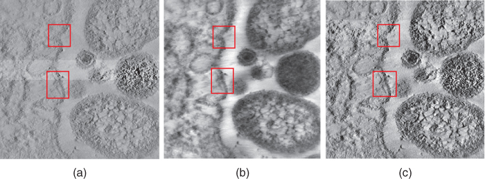
Montages showing one ![]() section of the volume reconstructed with the large datasets are presented in Figure 12.5. It clear that the quality of the image obtained by ASART is superior to the images obtained by WBP and SART. Since this dataset has a large noise level and no gold markers, the results of WBP and SART are so blurred that we can't catch the legible bilayer outlines of caveolae membrane structure, while the structure–phospholipid bilayer can be clearly observed in the result of ASART, as shown the red rectangles in Figure 12.5.
section of the volume reconstructed with the large datasets are presented in Figure 12.5. It clear that the quality of the image obtained by ASART is superior to the images obtained by WBP and SART. Since this dataset has a large noise level and no gold markers, the results of WBP and SART are so blurred that we can't catch the legible bilayer outlines of caveolae membrane structure, while the structure–phospholipid bilayer can be clearly observed in the result of ASART, as shown the red rectangles in Figure 12.5.
Figure 12.5 In the large dataset (![]() ), one of slices along the
), one of slices along the ![]() axis of the reconstructions of the caveolae by WBP (a), 50 iterations of SART (b), and 50 iterations of ASART (c). Caveolae membrane structures (indicated by the red rectangles) can be clearly observed in the result of ASART (c).
axis of the reconstructions of the caveolae by WBP (a), 50 iterations of SART (b), and 50 iterations of ASART (c). Caveolae membrane structures (indicated by the red rectangles) can be clearly observed in the result of ASART (c).
Also, we adopt a projection error ![]() criterion for the comparison of WBP, SART, and ASART in a practical situation.
criterion for the comparison of WBP, SART, and ASART in a practical situation. ![]() measures the mean discrepancy between the ray integral
measures the mean discrepancy between the ray integral ![]() and its calculated value
and its calculated value ![]() , defined as
, defined as
12.18 
where ![]() , and
, and ![]() is a
is a ![]() -dimensional vector whose
-dimensional vector whose ![]() th component is
th component is ![]() . In the 3D data reconstruction, the qualities of the reconstructions, with SART and ASART, respectively, have been evaluated using the measure
. In the 3D data reconstruction, the qualities of the reconstructions, with SART and ASART, respectively, have been evaluated using the measure ![]() . In general, a smaller projection error indicates a better reconstruction. The curves of the measure
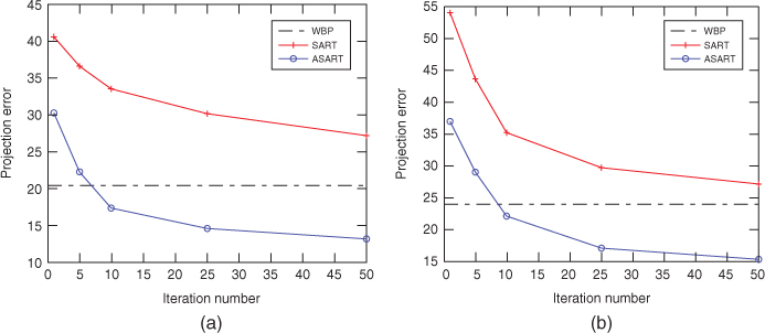
. In general, a smaller projection error indicates a better reconstruction. The curves of the measure ![]() versus the number of iterations are presented in Figure 12.6. As shown in that Figure 12.6,
versus the number of iterations are presented in Figure 12.6. As shown in that Figure 12.6, ![]() of the reconstructions with WBP remain constant, with the value of 20.35 and 23.94 in the small and large datasets, respectively. In the two different experiments,
of the reconstructions with WBP remain constant, with the value of 20.35 and 23.94 in the small and large datasets, respectively. In the two different experiments, ![]() of the reconstructions with ASART is smaller than that with SART in the same iterations. For the medium and large datasets, the values of
of the reconstructions with ASART is smaller than that with SART in the same iterations. For the medium and large datasets, the values of ![]() become smaller than that of WBP in 10 iterations. Consequently, it is shown that ASART has the advantage in dealing with extremely noisy conditions, and can obtain results better than those with WBP and SART.
become smaller than that of WBP in 10 iterations. Consequently, it is shown that ASART has the advantage in dealing with extremely noisy conditions, and can obtain results better than those with WBP and SART.
Figure 12.6 Plots of the projection errors ![]() versus the iteration numbers for the reconstructions of the caveolae using WBP, SART, and ASART at low resolution (a) and high resolution (b).
versus the iteration numbers for the reconstructions of the caveolae using WBP, SART, and ASART at low resolution (a) and high resolution (b).
12.5.3 Experimental Results of GPU Platform
To evaluate the multilevel parallel strategy, we have performed two sets of experiments to estimate the performance of an asynchronous communication scheme and the blob-ELLR data structure, respectively.
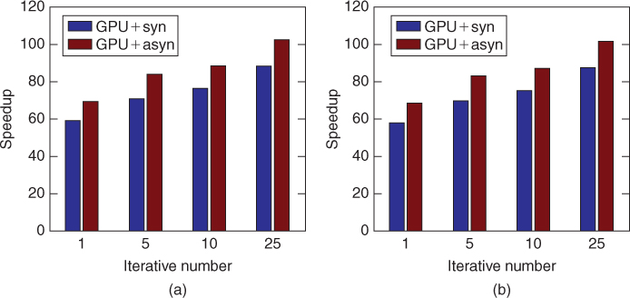
First, to estimate the performance of the asynchronous communication scheme, we implemented the blob-based iterative reconstruction algorithm (ASART) using the two experimental datasets on the Fermi platform. All the reconstructions adopt two methods separately: multi-GPUs with the synchronous communication scheme (viz., GPU+syn), and multi-GPUs with the asynchronous communication scheme (viz., GPU+asyn). In the experiments, the blob-ELLR developed in our work is used to storage the weighted matrix in the reconstruction. Figure 12.7 shows the speedups of the two communication schemes for different reconstructions iterative numbers (i.e., 1, 5, 10, 25) using the two datasets on the Tesla C2050 versus CPU. As shown in Figure 12.7, the speedups of GPU+asyn are larger than those of GPU+syn for two datasets. The asynchronous communication scheme exhibits excellent acceleration factors, reaching up to ![]() and
and ![]() for 25 iterations, on two datasets, respectively. In general, the asynchronous communication scheme provides better performance than the synchronous scheme for the reason of asynchronous overlap of communications and computations.
for 25 iterations, on two datasets, respectively. In general, the asynchronous communication scheme provides better performance than the synchronous scheme for the reason of asynchronous overlap of communications and computations.
Figure 12.7 Speedup factors of different iterations shown by both implementations on the Tesla C2050 and CPU.
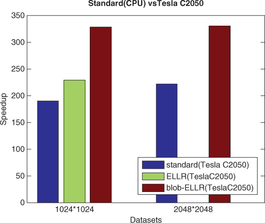
Further, to evaluate the bolb-ELLR data structure, we implemented and compared the blob-based iterative reconstruction method using standard matrix, ELLR matrix, and blob-ELLR matrix on the Fermi platform, respectively. Figure 12.8 compares the speedups against the method using standard matrix. To ensure a clear and brief description, we show the results of only two datasets for one iteration. Because of the limited memory, the ELLR matrix method for large dataset cannot be implemented on the Tesla C2050s. It is clearly seen that the blob-ELLR matrix method yields better speedups than the ELLR matrix method on the Tesla C2050s. Figure 12.9 compares the speedup factors of different methods on the Tesla C2050s over the standard method on the CPU for one iteration. It is clear that the blob-ELLR matrix method can reduce the memory requirement of the weighted matrix and yield the best performance compared with the ELLR matrix and the standard methods on GPU platforms.
Figure 12.8 Speedup factors of the different matrix methods (ELLR and blob-ELLR) for one iteration over the standard method on the Tesla C2050s.
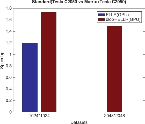
Figure 12.9 Speedup factors of the different matrix methods (standard, ELLR, and blob-ELLR) for one iteration on the Tesla C2050s.
12.6 Summary
In this study, we present an adaptive simulatneous algebraic reconstruction technique, named ASART, to obtain high-quality reconstructions, and developed a multilevel parallel strategy for a blob-based reconstruction algorithm on GPU platform. The contributions of ASART include a scheme MMAS for the organization and sequence of access to projections, a strategy AAR for parameter adjustment to correct the discrepancy between real projections and computed ones in each iteration, and a strategy CSS to process the weights for each view to reduce memory requirement and computation time. Experimental results show than ASART can obtain high-quality 3D reconstruction of ET under the condition of noisy and incomplete data. In the multilevel parallel strategy, the asynchronous communication scheme is used to minimize the idle GPU time. The blob-ELLR structure only needs nearly ![]() of the storage space in comparison with the ELLR storage structure and yields significant acceleration compared to the standard and ELLR matrix methods.
of the storage space in comparison with the ELLR storage structure and yields significant acceleration compared to the standard and ELLR matrix methods.
Acknowledgments
We would like to thank Professor Fei Sun in Institute of Biophysics, Chinese Academy of Sciences for providing the experimental datasets. This work supported by Chinese Academy of Sciences knowledge innovation key project (KGCX1-YW-13), and National Natural Science Foundation of China grant 61232001, 61202210 and 61103139.
References
1. Frank J, Three-Dimensional Electron Microscopy of Macromolecular Assemblies. Visualization of Biological Molecules in Their Native StateNature, Oxford Univ. Press, New York, 2006.
2. Henderson R, Realising the potential of electron cryomicroscopy, Q. Rev. Biophys. 37:3–13 (2004).
3. Zhou ZH, Towards atomic resolution structural determination by singleparticle cryo-electron microscopy realising the potential of electron cryomicroscopy, Curr. Opin. Struct. Biol. 18:218–228 (2008).
4. Lucic U, Foerster F, Baumeister W, Structural studies by electron tomography: From cells to molecules, Annu. Rev. Biochem. 74:833–865 (2004).
5. Robinson CV, Sali A, Baumeister W, The molecular sociology of the cell, Nature 450:973–982 (2007).
6. Marabini R, Rietzel E, Schroeder E, Herman G, Carazo J, Three-dimensional reconstruction from reduced sets of very noisy images acquired following a single-axis tilt schema: Application of a new three-dimensional reconstruction algorithm and objective comparison with weighted backprojection. The molecular sociology of the cell, J. Struct. Biol. 120:363–371 (1997).
7. Herman GT, Fundamentals of Computerized Tomography: Image Reconstruction from Projections, 2nd ed., Springer Press, London, 2009.
8. Fernandez JJ, Sorzano C, Marabini R, Carazo J, Image processing and 3-D reconstruction in electron microscopy, IEEE Signal Process. Mag. 23(3):84–94 (2006).
9. Radermacher M, Weighted back-projection methods, in Electron Tomography: Methods for Three-Dimensional Visualization of Structures in the Cell, 2nd ed., Springer, New York, 2006, Chap. 8.
10. Fernandez JJ, Lawrence A, Roca J, Garca J, Ellisman M, Carazo J, High performance electron tomography of complex biological specimens, J. Struct. Biol. 138:6–20 (2002).
11. Marabini R, Herman G, Carazo J, 3D reconstruction in electron microscopy using ART with smooth spherically symmetric volume elements (blobs), Ultramicroscopy 72:53–65 (1998).
12. Bilbao-Castro JR, Marabini R, Sorzano C, Garcia I, Carazo J, Fernandez JJ, Exploiting desktop supercomputing for three-dimensional electron microscopy reconstructions using ART with blobs, Ultramicroscopy 165:19–26 (2009).
13. Sorzano C, Marabini R, Boisset N, Rietzel E, Schroder R, Herman G, Carazo J, The effect of overabundant projection directions on 3D reconstruction algorithms, J. Struct. Biol. 133(2–3):108–118 (2001).
14. Castano-Diez D, Mueller H, Frangakis A, Implementation and performance evaluation of reconstruction algorithms on graphics processors, J. Struct. Biol. 157:288–295 (2007).
15. Censor Y, Finite series-expansion reconstruction methods, Proc. IEEE 71(3):409–419 (1983).
16. Lewitt RM, Alternative to voxels for image representation in iterative reconstruction algorithms, Phys. Med. Biol. 37:705–716 (1992).
17. Matej S, Lewitt RM, Efficient 3D grids for image-reconstruction using spherically-symmetrical volume elements, IEEE Trans. Nucl. Sci. 42:1361–1370 (1995).
18. Andersen AH, Kak AC, Simultaneous algebraic reconstruction technique (SART): A superior implementation of the ART algorithm, Ultrasonic Imag. 6:81–94 (1984).
19. Herman GT, Meyer L, Algebraic reconstruction can be made computationally efficient, IEEE Trans. Med. Imag. 12(3):600–609 (1993).
20. Frank J, Electron Tomography: Methods for Three-Dimensional Visualization of Structures in the Cell, 2nd ed., Springer, New York, 2006.
21. Guan H, Gordon R, A projection access order for speedy convergence of ART (algebraic reconstruction technique): A multilevel scheme for computed tomography, Phy. Med. Biol. 39:2005–2022 (1994).
22. Mueller K, Yagel R, Cornhill JF, The weighted-distance scheme: A globally optimizing projection ordering method for ART, IEEE Trans. Med. Imag. 16(2):223–230 (2002).
23. Kazantsev I, Matej S, Lewitt RM, Optimal ordering of projections using permutation matrices and angles between projection subspaces, Electron. Notes Discrete Math. 20:205–216 (2005).
24. Wenkai L, Adaptive algebraic reconstruction technique, Med. Phys. 31:3222–3230 (2004).
25. Wan XH, Zhang F, Liu ZY, Modified simultaneous algebraic reconstruction technique and its parallelization in cryo-electron tomography, Proc. Int. Conf. Parallel and Distributed Systems 2009, pp. 384–390.
26. Guan H, Gordon R, Computed tomography using algebraic reconstruction techniques (ARTs) with different projection access schemes: A comparison study under practical situations, Phys. Med. Biol. 41:1727–1743 (1996).
27. Guan H, Gordon R, Zhu Y, Combining various projection access schemes with the algebraic reconstruction technique for low-contrast detection in computed tomography, Phys. Med. Biol. 43:2413–2421 (1998).
28. Guan H, Yin FF, Zhu Y, Kim JH, Adaptive portal CT reconstruction: A simulation study, Med. Phys. 27:2209–2214 (2000).
29. Jiang M, Wang G, Convergence studies on iterative algorithms for image reconstruction, IEEE Trans. Med. Imag. 22:569–575 (2002).
30. Fernandez JJ, Carazo J, Garca I, Three-dimensional reconstruction of cellular structures by electron microscope tomography and parallel computing, J. Parallel Distrib. Comput. 64:285–300 (2004).
31. Bisseling RH, Parallel Scientific Computation, Oxford Univ. Press, New York, 2004.
32. Vazquez F, Garzon EM, Fernandez JJ, A new approach for sparse matrix vector product on NVIDIA GPUs, Concurr. Comput.: Pract. Exper. 23:815–826 (2011).
33. Vazquez F, Garzon EM, Fernandez JJ, A matrix approach to tomographic reconstruction and its implementation on GPUs, J. Struct. Biol. 170:146–151 (2010).
34. Sun S, Zhang K, Xu W, Wang G, Chen J, Sun F, 3D structural investigation of caveolae from porcine aorta endothelial cell by electron tomography, Progress Biochem. Biophys. 36(6):729–735 (2009).
35. Kremer JR, Mastronarde DN, McIntosh JR, Computer visualization of three-dimensional image data using IMOD, J. Struct. Biol. 116:71–76 (1996).