
Chapter 17
Protein Tertiary Model Assessment
17.1 Introduction
Protein structure prediction has been an important conundrum in the field of bioinformatics and theoretical chemistry because of its importance in medicine, drug design, biotechnology, and other areas. In structure biology, protein structures are often determined by techniques such as X-ray crystallography, NMR spectroscopy, and electron microscopy. A repository of these experimentally determined structures is organized as a centralized, proprietary databank called the Protein Data Bank (PDB). This databank is freely accessible on the Internet [1]. The generation of a protein sequence is much easier than the determination of protein structure. The structure of the protein gives much more insight about its function than its sequence. Therefore computational methods for the prediction of protein structure from its sequence have been developed. Ab initio prediction methods employ only the sequence of the protein based on the physical principles governing any molecular structure. Threading and homology modeling methods can build a 3D model for a protein of unknown structure from experimental structures of evolutionary related proteins. As long as a detailed physicochemical description of protein folding principles does not exist, structure prediction is the only method available to researchers to view the structure of some proteins. Experts agree that it is possible to construct high-quality full-length models for almost all single-domain proteins by using best possible template structure in PDB and state-of-the-art modeling algorithm [31–33]. This suggests that the current PDB structure universe may be approaching completion. So it all comes down to selecting that model in a pool of models.
We aim to obtain a learning algorithm that studies known structures from PDB and when given a protein model predicts whether it belongs to the same class as PBD structures. Since using a whole primary protein sequence to determine a 3D protein structure is very difficult, it is necessary to design new intelligent algorithms to find key features from a large pool of relevant features in biology and geometry to effectively evaluate 3D protein models. The central focus of this study is to develop and implement new granular decision machines to find biologically meaningful features for assessing 3D protein structures accurately and efficiently. This effort will lead to a better understanding of internal mechanism governing 3D protein structures such as how and why the key biological features and geometric features can dominate a 3D protein structure, and identify these critical sequence features and geometric features.
Solving this problem will help us study problems from different domains that have the same intensity of information. There are many complex and important application problems with huge geometric factors. A short list of common problems where geometry is a critical factor would include social and computer network structure, traffic analysis, and computer vision. Biomedical examples include 3D structural features of a protein that are directly related to basic functionality and are crucial for drug design.
17.2 Overview of Protein Model Assessment
Protein structure prediction methods are generally classified into three categories according to the necessity of a template structure used as a scaffold of a model of a target sequence: (1) homology modeling, (2) threading or fold recognition, and (3) ab initio methods. Method 1 is based on the observation that proteins with homologous sequence fold to almost identical structure. Therefore, when a highly homologous template structure for a target sequence is available in the PDB, the method can produce an accurate model with a root-mean-squared distance (RMSD) of 1–2 Å to its native structure. Conversely, the range of applications of homology modeling is relatively narrow because a template structure is necessary for calculation. Method 2 seeks a well-fitting known structure for a given target sequence, sometimes from a range of beyond-detectable sequence similarity.
An important task in both structure prediction and application is to evaluate the quality of a structure model. Half a century has passed since it was shown that an amino acid sequence of a protein determines its shape, but a method for reliable translation into the 3D structure still remains to be developed. So it is important to develop methods that determine the quality of a model. Since the early 1990s, a number of approaches have been developed to analyze correctness of protein structures and models. Traditional model evaluation methods use stereochemistry checks, molecular mechanical energy-based functions, and statistical potentials to tackle the problem. More recently, machine learning methods using algorithms such as neural networks (NNs) and support vector machines (SVMs) that are trained on structure models to predict model quality have been introduced [4]. There are various techniques available for determining the quality of a predicted model, either by comparing it with the native structure or with no knowledge of known structure. In the following paragraphs, the most familiar assessment techniques are categorized and the importance of each category is discussed.
These techniques can be divided into three basic categories according to their scoring strategy: local versus global, absolute versus relative, or single versus multiple (consensus or ranking methods). Some methods predict the quality of local regions such as distance between the position of a residue in a protein model and its native structure as supposedly predicting an overall score of a model. Some methods predict both local and global quality, such as Pcons [5]. Wallner and Elofsson's [6] Pcons is a consensus-based method capable of a quite reliable ranking of model sets for both easy and difficult targets. Pcons uses a metaserver approach (i.e., it combines results from several available well-established quality assessment methods) to calculate a quality score reflecting the average similarity of a model to the model ensemble, under the assumption that recurring structural patterns are more likely to be correct than those observed only rarely. It should be underscored that, while the consensus-based methods are useful in model ranking, they can be biased by the composition of the set and, in principle, are incapable of assessing the quality of a single model. This brings us to another category based on scoring: absolute score versus relative score. Relative scoring methods discriminate near-native structure from decoys; these methods are different from methods that produce absolute score. A relative score can only select or rank models but does not indicate the quality of a model, which is critical for using the model. The techniques could also be grouped according to the information needed for quality assessment. In prominent assessment approaches, 3D co-ordinates, sequence information, sequence alignment, alignment information, template, secondary structure information, and other features are generally used to judge quality. Model evaluation methods can be classified into single-model approach such as ProQ, Proq-LG, ProQ-MX, and MODCHECK and multimodel approaches such as clustering methods whose output depends on the number of input models. We can also group these techniques according to prediction accuracy, machine learning tools such as NNS and SVM, clustering, and consensus approaches. Some of these methods are used in critical assessment of structure prediction (CASP), as one of many analyses involved in assessment phase [37–39]. There are many methods that aim at finding the model quality, but very few come up with an absolute score using a single model and information from only its primary sequence and 3D coordinates [6, 7, 10, 11].
In the 2 years following CASP7, a considerable increase in method development in the area of model quality assessment can be observed. More than a dozen papers have been published on the subject, and 45 quality assessment methods, almost double the CASP7 number, have been submitted for evaluation to CASP8 [4, 9]. CASP evaluation is based on comparison of each model with the corresponding experimental structure. A GDT_TS score [12] is used in several CASP competitions, which is defined as average coverage of the target sequence of the substructure with four different distance thresholds. Other similar techniques obtain an absolute scoring by comparing the model to its experimental structure. A strikingly different domain involves assessment of the models with no known structure. Several methods have been proposed to solve this problem. Single-model approaches, including ProQ [5], ProQ-LG, ProQ-MX [10], and MODCHECK [13] assign a score to a single model, whereas multimodel approaches, such as clustering and consensus methods, require a large pool of models as inputs. These methods cannot be used to assess the quality of a single model. They may not reliably evaluate the quality of a small number of input models [4]. Machine learning methods such as neural networks and SVM that are trained on structure models predict model quality [11, 14, 15] differ by including the consensus-based features (i.e., incorporating in the analysis information from multiple models on the same target).
MODCHECK [13] places emphasis on benchmarking individual methods and also offers NN-based metatechniques that combine them. ModFOLD merges four orginal approaches in a program. Some of the more recent methods that make use of single-model, 3D coordinate information, and primary sequence to evaluate an absolute score for model quality assessment are ModelEvaluator [11] and Undertaker [16]. In ModelEvaluator [11] they use a normalized GDT_TS score with SVM regression to train SVM to learn a function that accurately maps input features. For a general overview of available techniques, please refer Table 17.1 [3, 5, 11–13, 16–19].
Table 17.1 Overview of Current Model Assessment Methods

Since models are not experimental structures determined with known accuracy but provide only predictions, it is vital to present the user with the corresponding estimates of model quality. Much is being done in this area, but further development of tools for reliable assessment of model quality is needed. Our approach is quite different from any recent study; we aim to classify the models into two classes: proteins and nonproteins. With thousands of protein structures available in the Protein Data Bank, it is possible to train a machine learning algorithm to study protein structure and predict whether a given model closely resembles these structures. From initial results we can say with some assurance that it is possible to achieve such a learning curve.
The amount and nature of information given to the machine learning system will have an impact on the final output regarding the quality measure of given 3D structure. There are various ways of representing a protein 3D structure, including a backbone sketch of the protein, the entire distance matrix of α-carbon atoms, a fractal dimension of the structure, and 3D information with its sequence data. These methods of representing protein structure are used mostly in comparison and classification problems and are widely studied and researched fields [20].
17.3 Design and Method
In order to classify whether a 3D object is a protein structure, the structure should be represented in machine-understandable format. In this methodology we represent each protein as one data vector. Each data vector should contain both structural and sequence information on that protein structure. For training and testing cycles using the machine learning algorithm, both positive and negative data vectors are needed. Positive vectors can be structures from the PDB database, as these structures are experimentally determined ones. Negative vectors are generated by misaligning the sequence and structure information, so that we have the wrong structure for a particular sequence. Different kernel methods and encoding schemes are used to observe their effectiveness in classifying proteins as either correct or incorrect. The goal here is to encode protein information in numerical form understandable by machine learning technique. The encoding is performed in the following order:
![]()
In the following two paragraphs, different methods for representing sequence and structure information are discussed. These are not the only methods for encoding protein information, but they are commonly used in other research domains, such as structure alignment, protein function classification, and protein secondary structure classification [21].
Protein sequence is a one-dimensional string of 20 different amino acids. To represent each amino acid, we can use one of the two very popular matrices. BLOSUM [blocks of (aminoacid) substitution matrix] is a substitution matrix. The scores measure the logarithm for the ratio of the likelihood of two amino acids appearing with a biological sense and the likelihood of the same amino acids appearing by chance. A positive score is given to the more likely substitutions; a negative score, to the less likely substitutions. The elements in this matrix are used as features for data vectors. For each amino acid there are 20 features to consider. Profile or position specific scoring matrix (PSSM) is a table that lists the frequencies of each amino acid in each position of protein sequence. Highly conserved positions receive high scores, and weakly conserved positions receive scores near zero. Profile, similar to the BLOSUM matrix, provides 20 features per amino acid. In preliminary studies both methods were used to encode sequence information. For IFID3 only BLOSUM matrix is used. This method is further illustrated in Figure 17.1.
Figure 17.1 Features of vector formation.

The distance matrix containing all pairwise distances between Cα atoms is one commonly used rotationally and translationally invariant representation of protein structure. This technique is used in DALI [20] for protein structure comparison by detecting spatial similarities. The major difficulty with distance matrices is that they cannot distinguish between right-handed and left-handed structures. Another evident problem with this method is computability, as there are too many parameters or attributes to optimize in the case of feature selection or optimization, which are important steps in the machine learning process. Two different simulations are performed for implementation of the design. The first simulation is the direct implementation of a larger dataset performed using support vectors technique. Because of some shortcomings in computational domain and poor prediction accuracy, the second simulation is considered. The second simulation uses a fuzzy decision tree to obtain better prediction accuracy.
The single positive vector is a single protein with its sequence information followed by its own structure information. The single negative vector has one protein's sequence information followed by another protein's structure information. For initial implementation we have considered two kernels: linear and Gaussian. Sequence information is represented using both BLOSUM and Profile to observe their individual performance. In case of structural information, only the distance matrix is considered to represent protein 3D structure. For example, to encode protein chain 1M56D of sequence length 51 using the Profile + distance matrix encoding scheme, its complete sequence and structure information has to be included. For every amino acid in the sequence we need to input 20 features corresponding to its position-specific score (PSSM or Profile), so the example protein will have 1020 (51*20) features to represent its sequence. For structure information we have to consider the (upper or lower) half of distance matrix, this will result in 1275 (51*50/2) features to represent its structure. In total, 2295 features are used to represent the protein chain. (Note: The entire sequence and structure details are considered; thus, for a protein of length 200 we will have 4000 features for sequence information and 19,900 for structure.) This will be a positive vector as it is from the PDB database. Negative vectors are generated by choosing sequence and structure information of two random proteins in a similar manner. For the BLOSUM matrix + distance matrix encoding scheme, the BLOSUM matrix is used instead of Profile.
The PDB entries are culled on the basis of their sequence length and relative homology using the PISCES server [22]. The culled list has ≤25% homology among different protein sequences. This will ensure that negative vectors are not false negative with highest probability.
17.4 Implementation Using Svm
Support vector machines (SVMs) are learning systems that use a hypothesis space of linear function in a high-dimensional feature space, trained with a learning algorithm from optimization theory that implements a learning bias derived from statistical learning theory. In supervised learning the learning machine is given a training set of examples (or inputs) with associated labels (or output values). Once the attributes vectors are available, a number of sets of hypotheses can be chosen for the problem. Among these, linear functions are best understood and simplest to apply. The development of learning algorithm became an important subfield of artificial intelligence, eventually forming the separate subject area of machine learning [21, 24, 23].
In this section, we discuss implementation of the proposed method using support vector machines. Different simulations are done to study the effectiveness of the selected machine learning technique in this data scenario. A specific set of PDB entries are culled according to their sequence length (200) and homology. Positive and negative data are obtained from the same set as discussed in the previous section.
17.4.1 Simulation 1
For this simulation, approximately 2000 PDB entries are culled from the entire PDB databank. These entries form the positive vectors for the learning system. The same number of negative vectors is generated by randomly selecting two PDB entries, one for sequence and other for structure information. The total number of training vectors hence obtained is 4670, and the number of testing vectors is 780. Results after the implementation are shown in Table 17.2.
Table 17.2 Encoding Scheme
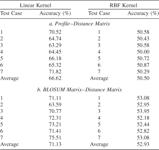
These results show sevenfold testing. From the tables we note that the BLOSUM matrix has better accuracy than does Profile. However, with the BLOSUM matrix for encoding, we note that Gaussian kernels are unable to give results comparable to those of the linear kernel. This might be due to incorrect optimization parameters. These results are not sufficient to warrant recommendation of any one encoding scheme or kernel; more simulations are required. Simulation 2 is performed to determine the effect of using all features as opposed to some randomly selected ones.
17.4.2 Simulation 2
From the simulation 1 results we note that the machine learning algorithm suffers from poor dimensionality, which affects computational efficiency and final accuracy. This could be due to the huge number of features considered in representing protein 3D structure. Feature reduction and selection techniques such as redesigning the feature, selecting an appropriate subset of features, or combining features could be considered to solve this problem. The training and testing datasets are constructed similarly to simulation 1.
To obtain this we will adopt a static scheduling algorithm that will schedule each training vector in a different processor. This scheduling will continue until the desired accuracy (equal to or greater than linear kernel accuracy with all features) or maximum number of tries is attained.
For effective analysis of the feature selection procedure, a different dataset was culled similar to one shown in previous section but with only 600 PDB entries. The number of training vectors thus obtained is 1030, and the number of testing vectors is 170. The results show the effectiveness of feature selection. The accuracies have also increased after feature selection.
Since the dataset considered here is different from that of simulation 1, we have calculated the sevenfold accuracy for this dataset. These results are shown in Table 17.3a. There is a drop in average percentage accuracies; this might be due to a lower number of training vectors.
Table 17.3 Accuracy Before and After Feature Selection
| Test | BLOSUM Matrix | Profile |
| Case | Encoding (%) | Encoding (%) |
| a. Before Feature Selection | ||
| 1 | 58.24 | 59.72 |
| 2 | 65.29 | 66.67 |
| 3 | 59.41 | 63.89 |
| 4 | 60.59 | 63.19 |
| 5 | 60.00 | 52.78 |
| 6 | 62.94 | 66.67 |
| 7 | 64.12 | 58.33 |
| Average | 61.51 | 61.60 |
| b. After Feature Selection | ||
| 1 | 60.50 | 64.58 |
| 2 | 66.47 | 68.75 |
| 3 | 62.55 | 66.67 |
| 4 | 65.29 | 65.28 |
| 5 | 63.53 | 58.33 |
| 6 | 65.29 | 69.44 |
| 7 | 67.06 | 63.89 |
| Average | 64.37 | 64.69 |
17.4.3 Feature Selection Algorithm
A simple algorithm is devised for purposes of feature selection. For a number of features to be selected, several percentages were tested to compare their performance with vectors that have all the features. After several trails 2% proved to be sufficient to obtain the same accuracy. To improve the speed of the algorithm, we used multiple processors. Each processor was scheduled to perform first the feature selection, followed by SVM training and then SVM testing. Once completed, the processor repeated the same task until the desired accuracy was obtained, or for a maximum number of attempts. The algorithm that we used consists in the following steps:
Table 17.3b lists the results obtained by using this above algorithm. The average has improved in both encoding schemes. Table 17.4 clearly shows the average accuracies of both encoding schemes before and after feature selection. This emphasizes the fact that all that features are not needed to make the binary decision. This leads us to consider other encoding schemes and representations of protein sequence and structure information. Other kernels should also be considered, as only the linear kernel has shown any real prediction ability [25].
Table 17.4 Comparison of Accuracies Before and After Feature Selection
| Encoding | Before Feature | After Feature |
| Scheme | Selection (%) | Selection (%) |
| BLOSUM matrix | 61.51 | 64.37 |
| Profile | 61.60 | 64.69 |
17.5 Implementation Using IFID3
Decision trees are one of the most popular machine learning techniques. They are known for their ability to represent the decision support information in a human-comprehensible form; however, they are recognized as a highly unstable classifier with respect to small changes in training data [26, 27]. One of the most popular algorithms for building decision trees is the Interactive Dichotomizer3 (ID3) algorithm proposed by Quinian in 1979 [26]. Generally, trees produced by ID3 (known as “crisp” decision trees) are sensitive to small changes in feature values and cannot handle data uncertainties caused by noise and/or measurement errors [27].
Nael Abu-halaweh and coworkers proposed an improved FID3 algorithm (IFID3) [28], the IFID3 integrates classification ambiguity and fuzzy information gain to select the branching attribute. The IFID3 algorithm outperformed the existing FID3 algorithm on a wide range of datasets. They also introduced an extended version of the IFID3 algorithm (EIFD3). EIFID3 extends IFID3 by introducing a new threshold on the membership value of a data instance to propagate down the decision tree from a parent node to any of its children nodes during the tree construction phase. Using the new threshold, a significant reduction in the number of rules produced, an improved accuracy, and a huge reduction in execution time are achieved. They automate the generation of the membership functions by two simple approaches. In the first approach the ranges of all numerical features in a dataset are divided evenly into an equal number of fuzzy sets. In the second approach, the dataset is clustered and the resulting cluster centers are used to generate fuzzy membership functions. These fuzzy decision trees were applied to the micro-RNA prediction problem; their results showed that fuzzy decision trees achieved a better accuracy than other machine learning approaches such as support vector machines (SVMs) and random forest (RF) [27].
With experimental results, they [27, 28] showed that the modified version of IFID3 produces better accuracy and achieves significant reduction in the number of resulting fuzzy rules. Overall, with their new fuzzy decision tree, they have improved the accuracy and execution time of induction algorithms by integrating fuzzy information gain and classification ambiguity to select the branching feature. By introducing a new threshold on the membership value of a data object to propagate down the decision tree from parent node to any of its child nodes, they have significantly reduced the number of fuzzy rules generated [28].
Both these features appeal to our dataset and objective of assessing models. The main reason for using this machine learning technique is the rule set that it generates. The rules will help in understanding the concepts and rules governing protein structure formation. Using these rules, we should be able to map out the path for correct protein structure models.
Three different datasets are considered. Each is a subset of the same dataset with a different number of proteins. Proteins from PDB are culled as discussed in Section 17.3. The proteins within a specific length range (150–200) are considered. Since there is a length variation among different proteins, for smaller proteins, a questionmark (?) is listed as an attribute value for positions where there is no amino acid. This kind of attribute definition is acceptable with IFID3 algorithms. This representation simply means that the attribute has no value or no meaning in the case considered here.
As mentioned earlier, IFID3 uses attribute classification ambiguity to select the branching attribute at the root node, and fuzzy information gain elsewhere. Given a dataset D with attributes A1, A2,…, An, based on the given parameter values, different fuzzy sets are formed for each attribute. The fuzzy ID3 algorithm requires the given dataset to be in a fuzzy form. In the present case, the dataset is not in fuzzy form but in continuous numerical form, so it needs to be fuzzified first. To obtain the optimal number of fuzzy sets, the number of fuzzy sets can be given as a parameter that needs to be tuned. The tree is built according to the given conditional parameters, and each node becomes a leaf node if the number of the dataset is less than a given threshold, if proportion of any class in the node is greater than the given fuzziness condition threshold, or if no additional attributes are available for classification [27, 28].
For our dataset we considered 10 fuzzy sets and triangular membership function for each attribute. The performance ratings of the tests are shown in Table 17.5. About 20 rules are generated for these datasets. There are three datasets, each with a different number of proteins. The first one has 100 proteins and hence 100 positive vectors and 100 negative vectors. Similarly, dataset 200 and 700 proteins have 200 positive vectors and 700 negative vectors, respectively. For sequence information, only BLOSUM matrix encoding is used. Table 17.7 shows sevenfold test results and their averages [29].
Table 17.5 Sevenfold Results Using IFID3
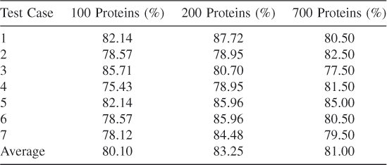
The prediction accuracy of IFID3 is much better when compared to SVM results. More simulations can be done with an increased number of proteins to check whether there is any improvement in prediction results.
17.6 Conclusion
Most aspects of experimental protein structure predictions process are difficult, time-consuming, expensive, labor-intensive, and problematic. Scientists have agreed that it is an impossible task to determine a complete set of all protein structures found in nature, since the number of proteins is much larger than the number of genes in an organism. On the other hand, scientists also believe that there are only a limited number of single-domain topologies, such that at some point the library of solved protein structure in PDB would be sufficiently complete and that the likelihood of finding a new fold is minimal. Earlier, although there were several thousand structures in PDB, most of these structures were not unique but rather were multiple variants of identical structure and sequence. So these models did not significantly expand our knowledge of protein structure space. Now experts believe that we have sufficient knowledge of protein structure space. This information is critical because it suggests that PDB structures provide a set from which other proteins can be modeled using computational techniques. These facts lead to the important task of estimating correctness of the prediction techniques and quality of protein models
Evaluating the accuracy of predicted models is critical for assessing structure prediction methods. This problem is not trivial; a large number of assessment measures have been proposed by various groups and have already become an active subfield of research. Most of these methods are normalized scoring functions that compare the given model to experimental structure. In this research we aim to obtain a binary classifier that studies structures from the PDB and classifies models as good or bad. The sheer volume of known structures available makes it possible to develop a machine learning system that studies protein structures and eventually predicts the quality of any new structure model. The most important task in this approach is represent to the protein 3D structure in the best possible manner and use an appropriate machine learning algorithm to obtain good assessment accuracy. The machine learning techniques considered in this chapter are support vector machines and fuzzy decision trees. To solve the protein model assessment problem, we employed attributes from the protein's sequence and structure.
To reduce the computational complexity of the program, we employed feature selection and parallel processing. We have implemented kernels to understand a complex 3D object and to determine whether the object represents a protein structure. By using an improved model of the fuzzy decision tree (IFID3), we could obtain prediction accuracy of >80%. The results look promising, but improvements in dataset a parameters could further improve the accuracy of prediction. Improvements such as making use of graph kernels, string kernels, kernel fusion methods, and decision fusion methods could further enhance the learning system. Also, these machines could be used to predict the results of previous CASP targets to test their accuracy in predicted models.
References
1. Berman HM, Westbrook J, Feng Z, Gilliland G, Bhat TN, Weissig H, Shindyalov IN, Bourne PE, The Protein Data Bank, Nucleic Acids Res. 28:235–242 (2000).
2. Berman HM, The Protein Data Bank: A historical perspective, Acta Crystallogr. A 64:88–95 (2008).
3. Zhang Y, Skolnick J, The protein structure prediction problem could be solved using current PDB library, Proc. Natl. Acad. Sci. USA 102:1029–1034 (2005).
4. Cozzetto D, Kryshtafovych A, Ceriani M, Tramontano A, Assessment of predictions in the model quality assessment category, Proteins 69(S8):175–183 (2007).
5. Wallner B, Fang H, Elofsson A, Automatic consensus-based fold recognition using pcons, proq, and pmodeller, Proteins 53:534–541 (2003).
6. Wallner B, Elofsson A, Can correct protein models be identified? Protein Sci. 12:1073–1086 (2003).
7. Moult J, A decade of CASP: Progress, bottlenecks and prognosis in protein structure prediction, Sci. Direct 15:285–289 (2005).
8. Siew N, Elofsson A, Rychlewski L, Fisher D, MaxSUb: An automated measure for the assessment of protein structure prediction quality, Bioinformatics 16(9):776–785 (2000).
9. Kihara D, Chen H, Yang YD, Quality assessment of protein structure models, Curr. Protein Peptide Sci. 10:216–228 (2009).
10. Wallner B, Elofsson A, Can correct regions in protein models be identified? Protein Sci. 15:900–913 (2006).
11. Wang Z, Tegge AN, Cheng J, Evaluating the absolute quality of a single protein model using structural features and support vector machines, Proteins: Struct., Funct., Bioinformatics 75(3):638–647 (2008).
12. Zemla A, Venclovas C, Moult J, Fidelis K, Processing and analysis of CASP3 protein structure prediction, Proteins (Suppl. 3):22–29 (1999).
13. Pettitt CS, Improving sequence-based fold recognition by using 3D model quality assessment, Bioinformatics 21(17):3509–3515 (2005).
14. Zhou H, Skolnick J, Protein model quality assessment prediction by combining fragment comparison and a consensus ca contact potential, Proteins 71:1211–1218 (2007).
15. Zhang Y, Skolnick J, SPICKER: A clustering approach to identify near-native protein folds, J. Comput. Chem. 25:865–871 (2004).
16. Karplus K, Katzman S, Shackleford G, Koeva M, Draper J, Barnes B, Soriano M, Hughey R, SAM-T04: What is new in protein structure prediction for CASP6, Proteins; 61:135–142 (2005).
17. Kajan L, Rychlewski L, Evaluation of 3D-jury on casp7 models, BMC Bioinformatics 8:304 (2007).
18. McGuffin LJ, The ModFOLD server for the quality assessment of protein structural models, Bioinformatics 24:586–587 (2008).
19. Zhou H, Skolnick J, Ab initio protein structure prediction using chunk—TASSER, Biophys. J. 93(5):1510–1518 (2007).
20. Holm L, Sander C, Protein structure comparison by alignment of distance matrices, J. Mol. Biol. 233:123–138 (1993).
21. Reyaz-Ahmed (Chida) A, Zhang YQ, Harrison R, Evolutionary neural SVM and complete SVM decision tree for protein secondary structure prediction, Int. J. Comput. Intell. Syst. 2(2):343–352 (2009).
22. Wang G, Dunbrack RL Jr PISCES: A protein sequence culling server, Bioinformatics 19:1589–1591 (2003).
23. Vapnik V, Corter C, Support vector networks, Machine Learn. 20:273–293 (1995).
24. Shawe-Taylor J, Cristianini N, Kernel Method for Pattern Analysis, Cambridge Univ. Press, (2004).
25. Joachims T, Making large-Scale SVM learning practical, in Schölkopf B, Burges C, Smola A, eds., Advances in Kernel Methods—Support Vector Learning, MIT Press, Cambridge, MA, 1999.
26. Reyaz-Ahmed (Chida) A, Harrison R, Zhang Y-Q, 3D protein model assessment using geometric and biological features, Proceedings of SEDM, Chengdu, 2010, June 23–25.
27. Quinian JR, Discovering rules by induction from large collection of examples, in Michi D, ed.: Expert Systems in Micro Electronics Age, Edinburgh Univ. Press, 1979.
28. Abu-Halaweh N, Harrison RW, Prediction and classifiction of real and pseudo microRNA precursors via data fuzzification and fuzzy decision tree. Proc. Int. Symp. Bioinformatics Research on Applications (ISBRA), Ft. Lauderdale 2009, pp. 323–334.
29. Abu-Halaweh N, Harrison RW, Rule set reduction in fuzzy decision trees, Proc. North American Fuzzy Information Processing Society Conf. (NAFIPS), Cincinnati 2009, pp. 1–4.
30. Reyaz-Ahmed (Chida) A, Abu-halaweh N, Harrison R, Zhang YQ, Protein model assessment via improved fuzzy decision tree, Proc. Int. Conf. Bioinformatics (BIOCOMP), Las Vegas, July 2010, pp. 12–15.
Bibliography
1. Abu-halaweh N, Harrison RW, Practical fuzzy decision trees, Proc. IEEE Symp. Computational Intelligence and Data Mining (ICTAI), Nashville 2000, pp. 203–206.
2. Chen XJ, Harrison R, Zhang Y-Q, Genetic fuzzy classification fusion of multiple SVMs for biomedical data, J. Intell. Fuzzy Syst. (special issue on evolutionary computing in bioinformatics) 18(6):527–541 (2007).
3. Fischer D, 3D-SHOTGUN: A novel, cooperative, fold-recognition meta-predictor, Proteins 51:434–441 (2003).
4. Lee K, Lee K, Lee J, Lee-Kwang H, A fuzzy decision tree induction method for fuzzy data, Proc. IEEE Conf. Fuzzy Systems (FUZZ-IEEE 99), Seoul, 1999, vol. 1, pp. 16–25.
5. McGuffin L, Bryson K, Jones D, What are the baselines for protein fold recognition? Bioinformatics 17:63–72 (2001).
6. Qiu J, Sheffler W, Baker D, Noble WS, Ranking predicted protein structures with support vector regression, Proteins 71:1175–1182 (2008).
7. Quinian JR, Introduction of decision trees, Machine Learn. 1:81–106 (1986).
8. Tang YC, Zhang Y-Q, Huang Z, Development of two-stage SVM-RFE gene selection strategy for microarray expression data analysis, IEEE/ACM Trans. Comput. Biol. Bioinformatics 4(3):365–381 (July–Sept. 2007).
9. Zhang Y, Progress and challenges in protein structure prediction, Curr. Opin. Struct. Biol. 18(3):342–348 (June 2008).