
Chapter 16
Fractal Related Methods for Predicting Protein Structure Classes and Functions
16.1 Introduction
The molecular function of a protein can be inferred from the protein's structure information [1]. It is well known that an amino acid sequence partially determines the eventual three-dimensional structure of a protein, and the similarity at the protein sequence level implies similarity of function [2, 3]. The prediction of protein structure and function from amino acid sequences is one of the most important and challenge problems in molecular biology.
Protein secondary structure, which is a summary of the general conformation and hydrogen bonding pattern of the amino acid backbone [4, 5], provides some knowledge to further simplify the complicated 3D structure prediction problem. Hence an intermediate but useful step is to predict the protein secondary structure. Since the 1970s, many methods have been developed for predicting protein secondary structure (see the more recent references cited in Ref. [6]).
Four main classes of protein structures, based on the types and arrangement of their secondary structural elements, were recognized [7]: (1) the ![]() helices, (2) the
helices, (2) the ![]() strands, and (3) those with a mixture of
strands, and (3) those with a mixture of ![]() and
and ![]() shapes denoted as
shapes denoted as ![]() and
and ![]() . This structural classification has been accepted and widely used in protein structure and function prediction. As a consequence, it has become an important problem and can help build protein database and predict protein function. In fact, Hou et al. [1] (see also a short report published in Science [8]) constructed a map of the protein structure space using the pairwise structural similarity of 1898 protein chains. They found that the space has a defining feature showing these four classes clustered together as four elongated arms emerging from a common center. A review by Chou [9] described the development of some existing methods for prediction of protein structural classes. Proteins in the same family usually have similar functions. Therefore family identification is an important problem in the study of proteins.
. This structural classification has been accepted and widely used in protein structure and function prediction. As a consequence, it has become an important problem and can help build protein database and predict protein function. In fact, Hou et al. [1] (see also a short report published in Science [8]) constructed a map of the protein structure space using the pairwise structural similarity of 1898 protein chains. They found that the space has a defining feature showing these four classes clustered together as four elongated arms emerging from a common center. A review by Chou [9] described the development of some existing methods for prediction of protein structural classes. Proteins in the same family usually have similar functions. Therefore family identification is an important problem in the study of proteins.
Because similarity in the protein sequence normally implies similarity of function and structure, the similarities of protein sequences can therefore be used to detect the biological function and interaction of proteins [10]. It is necessary to enrich the concept and context of similarity, because some proteins with low sequence identity may have similar tertiary structure and function [11].
Fractal geometry provides a mathematical formalism for describing complex spatial and dynamical structures [12, 13]. Fractal methods are known to be useful for detection of similarity. Traditional multifractal analysis is a useful way to characterize the spatial heterogeneity of both theoretical and experimental fractal patterns [14]. More recently it has been applied successfully in many different fields, including time series analysis and financial modeling [15]. Some applications of fractal methods to DNA sequences are provided in References [16–18] and references cited therein.
Wavelet analysis, recurrence quantification analysis (RQA), and empirical mode decomposition (EMD) are related to fractal methods in nonlinear sciences. Wavelet analysis is a useful tool in many applications such as noise reduction, image processing, information compression, synthesis of signals, and the study of biological data. Wavelets are mathematical functions that decompose data into different frequency components and then describe each component with a resolution matched to its scale [19, 20]. The recurrence plot (RP) is a purely graphical tool originally proposed by Eckmann et al. [21] to detect patterns of recurrence in the data. RQA is a relatively new nonlinear technique introduced by Zbilut and Webber [22, 23] that can quantify the information supplied by RP. The traditional EMD for data, which is a highly adaptive scheme serving as a complement to Fourier and wavelet transforms, was originally proposed by Huang et al. [24]. In EMD, a complicated dataset is decomposed into a finite, often small, number of components called intrinsic mode functions (IMFs). Lin et al. [25] presented a new approach to EMD. This method has been used successfully in many applications in analyzing a diverse range of datasets in biological and medical sciences, geophysics, astronomy, engineering, and other fields [26, 27].
Fractal methods have been used to study proteins. Their applications include fractal analysis of the proton exchange kinetics [28], chaos game representation of protein structures [29], sequences based on the detailed HP model [30, 31], fractal dimension of protein mass [32], fractal properties of protein chains [33], fractal dimensions of protein secondary structures [34], multifractal analysis of the solvent accessibility of proteins [35], and the measure representation of protein sequences [36]. The wavelet approach has been used for prediction of secondary structures of proteins [37–45]. Chen et al. [41] predicted the secondary structure of a protein by the continuous wavelet transform (CWT) and Chou–Fasman method. Marsolo et al. [42] combined the pairwise distance with wavelet decomposition to generate a set of coefficients and capture some features of proteins. Qiu et al. [43] used the continuous wavelet transform to extract the position of the ![]() helices and short peptides with specialscales. Rezaei et al. [44] applied wavelet analysis to membrane proteins. Pando et al. [45] used the discrete wavelet transform to detect protein secondary structures. Webber et al. [46] defined two independent variables to elucidate protein secondary structures based on the RQA of coordinates of
helices and short peptides with specialscales. Rezaei et al. [44] applied wavelet analysis to membrane proteins. Pando et al. [45] used the discrete wavelet transform to detect protein secondary structures. Webber et al. [46] defined two independent variables to elucidate protein secondary structures based on the RQA of coordinates of ![]() -carbon atoms. The variables can describe the percentage of
-carbon atoms. The variables can describe the percentage of ![]() carbons that are composed of an
carbons that are composed of an ![]() helix and a
helix and a ![]() sheet, respectively. The ability of RQA to deal with protein sequences was reviewed by Giuliani et al. [47]. The IMFs obtained by the EMD method were used to discover similarities of protein sequences, and the results showed that IMFs may reflect the functional identities of proteins [48, 49].
sheet, respectively. The ability of RQA to deal with protein sequences was reviewed by Giuliani et al. [47]. The IMFs obtained by the EMD method were used to discover similarities of protein sequences, and the results showed that IMFs may reflect the functional identities of proteins [48, 49].
More recently, the authors used the fractal methods and related wavelet analysis, RQA and EMD methods to study the prediction of protein structure classes and functions [50–54]. In this chapter, we review the methods and results in these studies.
16.2 Methods
16.2.1 Measure Representation Based on the Detailed HP Model and Six-Letter Model
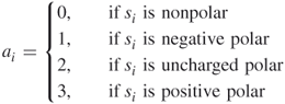
The detailed HP model was proposed by Yu et al. [30]. In this model, 20 different kinds of amino acids are divided into four classes: nonpolar, negative polar, uncharged polar, and positive polar. The nonpolar class consists of the eight residues ALA, ILE, LEU, MET, PHE, PRO, TRP, and VAL; the negative polar class consists of the two residues ASP and GLU; the uncharged polar class is made up of the seven residues ASN, CYS, GLN, GLY, SER, THR, and TYR; and the remaining three residues ARG, HIS, and LYS designate the positive polar class.
For a given protein sequence ![]() with length
with length ![]() , where
, where ![]() is one of the 20 kinds of amino acids for
is one of the 20 kinds of amino acids for ![]() we define
we define
This results in a sequence ![]() , where
, where ![]() is a letter of the alphabet
is a letter of the alphabet ![]() . The mapping (16.1) is called the detailed HP model [30].
. The mapping (16.1) is called the detailed HP model [30].
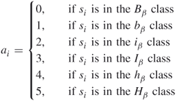
According to Chou and Fasman [55], the 20 different kinds of amino acids are divided into six classes: strong ![]() , former (
, former (![]() );
); ![]() former (
former (![]() );weak
);weak ![]() , former (
, former (![]() );
); ![]() indifferent (
indifferent (![]() );
); ![]() breaker (
breaker (![]() ); and strong
); and strong ![]() breaker (
breaker (![]() ). The
). The ![]() class consists of the three residues Met, Val, and IlE; the
class consists of the three residues Met, Val, and IlE; the ![]() class consists of the seven residues Cys, Tyr, Phe, Gln, Leu, Thr, and Trp; the
class consists of the seven residues Cys, Tyr, Phe, Gln, Leu, Thr, and Trp; the ![]() class consists of the residue Ala; the
class consists of the residue Ala; the ![]() class consists of the three residues Arg, Gly, and Asp; the
class consists of the three residues Arg, Gly, and Asp; the ![]() class is made up of the five residues Lys, Ser, His, Asn, and Pro; and the remaining residue Glu constitutes the
class is made up of the five residues Lys, Ser, His, Asn, and Pro; and the remaining residue Glu constitutes the ![]() class.
class.
For a given protein sequence ![]() with length
with length ![]() , where
, where ![]() is one of the 20 kinds of amino acids for
is one of the 20 kinds of amino acids for ![]() , we define
, we define
This results in a sequence ![]() , where
, where ![]() is a letter of the alphabet
is a letter of the alphabet ![]() . The mapping (16.2) is called the six-letter model [51].
. The mapping (16.2) is called the six-letter model [51].
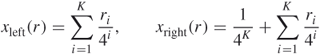
Here we call any string made up of ![]() letters from the set
letters from the set ![]() (for the detailed HP model) or
(for the detailed HP model) or ![]() (for the six-letter model) a
(for the six-letter model) a ![]() -string. For a given
-string. For a given ![]() , there are in total
, there are in total ![]() or
or ![]() different
different ![]() strings. In order to count the number of
strings. In order to count the number of ![]() strings in a sequence
strings in a sequence ![]() from a protein sequence
from a protein sequence ![]() , we need
, we need ![]() or
or ![]() counters. We divide the interval
counters. We divide the interval ![]() into
into ![]() or
or ![]() disjoint subintervals, and use each subinterval to represent a counter. For
disjoint subintervals, and use each subinterval to represent a counter. For ![]() which is a substring with length
which is a substring with length ![]() , we define
, we define
For ![]() ,
, ![]() ,
, ![]() which is a substring with length
which is a substring with length ![]() , we define
, we define
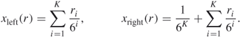
We then use the subinterval ![]() to represent substring
to represent substring ![]() . Let
. Let ![]() be the number of times that a substring
be the number of times that a substring ![]() with length
with length ![]() appears in the sequence
appears in the sequence ![]() (when we count these numbers, we open a reading frame with width
(when we count these numbers, we open a reading frame with width ![]() and slide the frame one amino acid each time). We define
and slide the frame one amino acid each time). We define
16.5 ![]()
to be the frequency of substring ![]() . It follows that
. It follows that ![]() . We can now define a measure
. We can now define a measure ![]() on
on ![]() by
by ![]() , where
, where
16.6 ![]()
when ![]() defined by (16.3). We define a measure
defined by (16.3). We define a measure ![]() on
on ![]() by
by ![]() , where
, where
16.7 ![]()
when ![]() defined by (16.4). We see that
defined by (16.4). We see that ![]() and
and ![]() . We call
. We call ![]() and
and ![]() the measure representation of the protein sequence corresponding to the given
the measure representation of the protein sequence corresponding to the given ![]() based on the detailed HP model and the six-letter model, respectively.
based on the detailed HP model and the six-letter model, respectively.
16.2.2 Measures and Time Series Based on the Physicochemical Features of Amino Acids
Measured in kcal/mol, the hydrophobic free energies of the 20 amino acids are ![]() ,
, ![]() ,
, ![]() ,
, ![]() ,
, ![]() ,
, ![]() ,
, ![]() ,
, ![]() ,
, ![]() ,
, ![]() ,
, ![]() ,
, ![]() ,
, ![]() ,
, ![]() ,
, ![]() ,
, ![]() ,
, ![]() ,
, ![]() ,
, ![]() , and
, and ![]() [39].
[39].
The solvent accessibility (SA) values for solvent exposed area ![]() are
are ![]() ,
, ![]() ,
, ![]() ,
, ![]() ,
, ![]() ,
, ![]() ,
, ![]() ,
, ![]() ,
, ![]() ,
, ![]() ,
, ![]() ,
, ![]() ,
, ![]() ,
, ![]() ,
, ![]() ,
, ![]() ,
, ![]() ,
, ![]() ,
, ![]() , and
, and ![]() [56].
[56].
The Schneider–Wrede scale (SWH) values of the 20 kinds of amino acids are ![]() ,
, ![]() ,
, ![]() ,
, ![]() ,
, ![]() ,
, ![]() ,
, ![]() ,
, ![]() ,
, ![]() ,
, ![]() ,
, ![]() ,
, ![]() ,
, ![]() ,
, ![]() ,
, ![]() ,
, ![]() ,
, ![]() ,
, ![]() ,
, ![]() , and
, and ![]() [47]. Yang et al. [51] added a constant 12.30 to these values to make all the 20 values nonnegative, yielding the revised Schneider–Wrede scale hydrophobicity (RSWH).
[47]. Yang et al. [51] added a constant 12.30 to these values to make all the 20 values nonnegative, yielding the revised Schneider–Wrede scale hydrophobicity (RSWH).
Rose et al. [57] proposed different measures of hydrophobicity of proteins. They gave four kinds of values for surface area and hydrophobicity of each amino acid. We use ![]() , the stochastic standard state accessibility, that is, the solvent accessible surface area (SASA) of a residue in standard state. The SASA of the 20 kinds of amino acids are
, the stochastic standard state accessibility, that is, the solvent accessible surface area (SASA) of a residue in standard state. The SASA of the 20 kinds of amino acids are ![]() ,
, ![]() ,
, ![]() ,
, ![]() ,
, ![]() ,
, ![]() ,
, ![]() ,
,![]() ,
, ![]() ,
, ![]() ,
, ![]() ,
, ![]() ,
, ![]() ,
, ![]() ,
, ![]() ,
, ![]() ,
, ![]() ,
, ![]() ,
, ![]() , and
, and ![]() .
.
Each amino acid can also be represented by the value of the volume of sidechains of amino acids [58]. These values are ![]() ,
, ![]() ,
, ![]() ,
, ![]() ,
, ![]() ,
, ![]() ,
, ![]() ,
, ![]() ,
, ![]() ,
, ![]() ,
, ![]() ,
, ![]() ,
, ![]() ,
, ![]() ,
, ![]() ,
, ![]() ,
, ![]() ,
, ![]() ,
, ![]() , and
, and ![]() .
.
We convert each amino acid according to hydrophobic free energy, SA, RSWH, SASA, and volume of sidechains along the protein sequence to calculate five different numerical sequences, and view them as time series.
Let ![]() ,
, ![]() , be the time series with length
, be the time series with length ![]() . First, we define
. First, we define ![]() as the frequency of
as the frequency of ![]() . It follows that
. It follows that ![]() . Now we can define a measure
. Now we can define a measure ![]() on the interval
on the interval ![]() by
by ![]() , where
, where
16.8 
We denote the interval ![]() by
by ![]() . It is seen that
. It is seen that ![]() and
and ![]() . We call
. We call ![]() the measure for the time series.
the measure for the time series.
16.2.3  -Curve Representation of Proteins
The concept of ![]() -curve representation of a DNA sequence was first proposed by Zhang and Zhang [59]. We propose a similar concept for proteins [50]. Once we get the sequence
-curve representation of a DNA sequence was first proposed by Zhang and Zhang [59]. We propose a similar concept for proteins [50]. Once we get the sequence ![]() for a protein, where
for a protein, where ![]() is a letter of the alphabet
is a letter of the alphabet ![]() as in Section 16.2.1, we can define the Z-curve representation of this protein as follows. This
as in Section 16.2.1, we can define the Z-curve representation of this protein as follows. This ![]() curve consists of a series of nodes
curve consists of a series of nodes ![]()
![]() , whose coordinates are denoted by
, whose coordinates are denoted by ![]() ,
, ![]() and
and ![]() . These coordinates are defined as
. These coordinates are defined as
16.9 
where ![]() denote the number of occurrences of the symbols 0,1,2,3 in the prefix
denote the number of occurrences of the symbols 0,1,2,3 in the prefix ![]() , respectively, and
, respectively, and ![]() . The connection of nodes
. The connection of nodes ![]() to one another by straight lines is defined as the Z-curve representation of this protein. We then define
to one another by straight lines is defined as the Z-curve representation of this protein. We then define
16.10 
where ![]() ,
, ![]() , and
, and ![]() can only have values 1 and
can only have values 1 and ![]() .
.
16.2.4 Chaos Game Representation of Proteins and Related Time Series
Chaos game representation (CGR) of protein structures was first proposed by Fiser et al. [29]. We denote this CGR by 20-CGR as 20 kinds of letters are used to represent protein sequences. Later Basu et al. [60] and Yu et al. [31] proposed other kinds of CGRs for proteins, in which 12 and 4 kinds of letters were used for protein sequences, respectively. We denote them by 12-CGR and 4-CGR.
16.2.4.1 Reverse Encoding for Amino Acids
It is known that there are several kinds of coded methods for some amino acids. As a result, there should be many possible nucleotide sequences for one given protein sequence. We have used [52], the encoding method proposed by Deschavanne and Tufféry [61], which is listed in Table 1 of our study [52]. Deschavanne and Tufféry [61] explained that the rationale for the choice of this fixed code is to keep a balance in base composition so as to maximize the difference between the amino acid codes.
After one protein sequence is transformed into nucleotide sequences, we can use the CGR of nucleotide sequences [62] to analyze it; the CGR obtained is abbreviated AAD-CGR (amino acids to DNA CGR). The CGR for a nucleotide sequence is defined on the square ![]() , where the four vertices correspond to the four letters A, C, G, and T: the first point of the plot is placed half way between the center of the square and the vertex corresponding to the first letter of the nucleotide sequence; the
, where the four vertices correspond to the four letters A, C, G, and T: the first point of the plot is placed half way between the center of the square and the vertex corresponding to the first letter of the nucleotide sequence; the ![]() th point of the plot is then placed half way between the
th point of the plot is then placed half way between the ![]() th point and the vertex corresponding to the
th point and the vertex corresponding to the ![]() th letter. The plot is then called the CGR of the nucleotide sequence, or the AAD-CGR of the protein sequence.
th letter. The plot is then called the CGR of the nucleotide sequence, or the AAD-CGR of the protein sequence.
We can decompose the AAD-CGR plot into two time series [52]. Any point in the AAD-CGR plot is determined by two coordinates: ![]() and
and ![]() coordinates. Because the AAD-CGR plot can be uniquely reconstructed from these two time series, all the information stored in the AAD-CGR plot is contained in the time series, and the information in the AAD-CGR plot comes from the primary sequence of proteins. Therefore, any analysis of the two time series is equivalent to an indirect analysis of the protein primary sequence. It is possible that such analysis provides better results than direct analysis of the protein primarysequences.
coordinates. Because the AAD-CGR plot can be uniquely reconstructed from these two time series, all the information stored in the AAD-CGR plot is contained in the time series, and the information in the AAD-CGR plot comes from the primary sequence of proteins. Therefore, any analysis of the two time series is equivalent to an indirect analysis of the protein primary sequence. It is possible that such analysis provides better results than direct analysis of the protein primarysequences.
16.2.5 Time Series Based on 6-Letter Model, 12-Letter Model, and 20-Letter Model
According to the 6-letter model, the protein sequence can be represented by a numerical sequence ![]() ; here
; here ![]() for each
for each ![]() .
.
We now analogously define a 12-letter model and a 20-letter model. With the idea of chaos game representation based on a 12-sided regular polygon [60], we define the 12-letter model as ![]() ,
, ![]() ,
, ![]() ,
, ![]() ,
, ![]() ,
, ![]() ,
, ![]() ,
, ![]() ,
, ![]() ,
, ![]() ,
, ![]() ,
, ![]() ,
, ![]() ,
, ![]() ,
, ![]() ,
, ![]() ,
, ![]() ,
, ![]() ,
, ![]() , and
, and ![]() according to the order of vertices on the 12-sided regular polygon to represent these amino acids.
according to the order of vertices on the 12-sided regular polygon to represent these amino acids.
The 20-letter model can be similarly defined as ![]() ,
, ![]() ,
, ![]() ,
, ![]() ,
, ![]() ,
, ![]() ,
, ![]() ,
, ![]() ,
, ![]() ,
, ![]() ,
, ![]() ,
, ![]() ,
, ![]() ,
, ![]() ,
, ![]() ,
, ![]() ,
, ![]() ,
, ![]() ,
, ![]() , and
, and ![]() according to the dictionary order of the 3-letter representation of each amino acid listed in Brown's treatise [63].
according to the dictionary order of the 3-letter representation of each amino acid listed in Brown's treatise [63].
These three models can be used to convert a protein sequence into three different numerical sequences (and also can be viewed as time series).
16.2.6 Iterated Function Systems Model
In order to simulate the measure representation of a protein sequence, we proposed use of the iterated function systems (IFS) model [30]. IFS is the acronym assigned by Barnsley and Demko [64] originally to a system of contractive maps ![]() . Let
. Let ![]() be a compact set in a compact metric space,
be a compact set in a compact metric space, ![]() and
and
![]()
Then ![]() is called the attractor of the IFS. The attractor is usually a fractal set and the IFS is a relatively general model to generate many well-known fractal sets such as the Cantor set and the Koch curve. Given a set of probabilities
is called the attractor of the IFS. The attractor is usually a fractal set and the IFS is a relatively general model to generate many well-known fractal sets such as the Cantor set and the Koch curve. Given a set of probabilities ![]() , we pick an
, we pick an ![]() and define the iteration sequence
and define the iteration sequence
![]()
where the indices ![]() are chosen randomly and independently from the set
are chosen randomly and independently from the set ![]() with probabilities
with probabilities ![]() . Then every orbit
. Then every orbit ![]() is dense in the attractor
is dense in the attractor ![]() [64]. For
[64]. For ![]() sufficiently large, we can view the orbit
sufficiently large, we can view the orbit ![]() as an approximation of
as an approximation of ![]() . This process is called chaos game.
. This process is called chaos game.
Let ![]() the characteristic function for the Borel subset
the characteristic function for the Borel subset ![]() , then, from the ergodic theorem for IFS [64], the limit
, then, from the ergodic theorem for IFS [64], the limit
exists. The measure ![]() is the invariant measure of the attractor of the IFS. In other words,
is the invariant measure of the attractor of the IFS. In other words, ![]() is the relative visitation frequency of
is the relative visitation frequency of ![]() during the chaos game. A histogram approximation of the invariant measure may then be obtained by counting the number of visits made to each pixel.
during the chaos game. A histogram approximation of the invariant measure may then be obtained by counting the number of visits made to each pixel.
The coefficients in the contractive maps and the probabilities in the IFS model are the parameters to be estimated for a real measure that we want to simulate. A moment method [30, 65] can be used to perform this task.
From the measure representation of a protein sequence based on the detailed HP model, it is logical to choose ![]() and
and
in the IFS model. For a given measure representation of a protein sequence based on the detailed HP model, we obtain the estimated values of the probabilities ![]() by solving an optimization problem [65]. Using the estimated values of the probabilities, we can use the chaos game to generate a histogram approximation of the invariant measure of the IFS that can be compared with the real measure representation of the protein sequence.
by solving an optimization problem [65]. Using the estimated values of the probabilities, we can use the chaos game to generate a histogram approximation of the invariant measure of the IFS that can be compared with the real measure representation of the protein sequence.
16.2.7 Detrended Fluctuation Analysis
The exponent in a detrended fluctuation analysis can be used to characterize the correlation of a time series [17, 18]. We view ![]() ,
, ![]() , and
, and ![]()
![]() in the
in the ![]() -curve representation of proteins as time series. We denotethis time series by
-curve representation of proteins as time series. We denotethis time series by ![]() . First, the time series is integrated as
. First, the time series is integrated as ![]() , where
, where ![]() is the average over the whole time period. Next, the integrated time series is divided into boxes of equal length
is the average over the whole time period. Next, the integrated time series is divided into boxes of equal length ![]() . In each box of length
. In each box of length ![]() , a linear regression is fitted to the data by least squares, representing the trend in that box. We denote the
, a linear regression is fitted to the data by least squares, representing the trend in that box. We denote the ![]() coordinate of the straight-line segments by
coordinate of the straight-line segments by ![]() . We then detrend the integrated time series
. We then detrend the integrated time series ![]() by subtracting the local trend
by subtracting the local trend ![]() in each box. The root-mean-square fluctuation of this integrated and detrended time series is computed as
in each box. The root-mean-square fluctuation of this integrated and detrended time series is computed as
16.11 
Typically, ![]() increases with box size
increases with box size ![]() . A linear relationship on a log–log plot indicates the presence of scaling
. A linear relationship on a log–log plot indicates the presence of scaling ![]() . Under such conditions, the fluctuations can be characterized by the scaling exponent
. Under such conditions, the fluctuations can be characterized by the scaling exponent ![]() , the slope of the line in the regression
, the slope of the line in the regression ![]() against
against ![]() . For uncorrelated data, the integrated time series
. For uncorrelated data, the integrated time series ![]() corresponds to a random walk, and therefore,
corresponds to a random walk, and therefore, ![]() . A value of
. A value of ![]() indicates the presence of long memory so that, for example, a large value is likely to be followed by large values. In contrast, the range
indicates the presence of long memory so that, for example, a large value is likely to be followed by large values. In contrast, the range ![]() indicates a different type of power-law correlation such that positive and negative values of the time series are more likely to alternate. We consider the exponents
indicates a different type of power-law correlation such that positive and negative values of the time series are more likely to alternate. We consider the exponents ![]() for the
for the ![]() ,
, ![]() , and
, and ![]()
![]() of the
of the ![]() -curve representation of protein sequences as candidates constructing parameter spaces for proteins in this chapter. These exponents are denoted by
-curve representation of protein sequences as candidates constructing parameter spaces for proteins in this chapter. These exponents are denoted by ![]() ,
, ![]() , and
, and ![]() respectively.
respectively.
16.2.8 Ordinary Multifractal Analysis
The most common algorithms of multifractal analysis are the so-called fixed-size box counting algorithms [16]. In the one-dimensional case, for a given measure ![]() with support
with support ![]() , we consider the partition sum
, we consider the partition sum
16.12 ![]()
with ![]() , where the sum runs over all different nonempty boxes
, where the sum runs over all different nonempty boxes ![]() of a given side
of a given side ![]() in a grid covering of the support
in a grid covering of the support ![]() , that is,
, that is, ![]() . The exponent
. The exponent ![]() is defined by
is defined by
and the generalized fractal dimensions of the measure are defined as
16.14 ![]()
16.15 ![]()
where ![]() . The generalized fractal dimensions are numerically estimated through a linear regression of
. The generalized fractal dimensions are numerically estimated through a linear regression of ![]() against
against ![]() for
for ![]() , and similarly through a linear regression of
, and similarly through a linear regression of ![]() against
against ![]() for
for ![]() . The value
. The value ![]() is called the information dimension and
is called the information dimension and ![]() , the correlation dimension.
, the correlation dimension.
The concept of phase transition in multifractal spectra was introduced in studies of logistic maps, Julia sets, and other simple systems. By following the thermodynamic formulation of multifractal measures, Canessa [66] derived an expression for the analogous specific heat as
16.16 ![]()
He showed that the form of ![]() resembles a classical phase transition at a critical point for financial time series.
resembles a classical phase transition at a critical point for financial time series.
The singularities of a measure are characterized by the Lipschitz–Hölder exponent ![]() which is related to
which is related to ![]() by
by
Substitution of Equation (16.13) into Equation (16.17) yields
16.18 ![]()
Again the exponent ![]() can be estimated through a linear regression of
can be estimated through a linear regression of
against ![]() [35]. The multifractal spectrum
[35]. The multifractal spectrum ![]() versus
versus ![]() can be calculated according to the relationship
can be calculated according to the relationship ![]() .
.
16.2.9 Analogous Multifractal Analysis
The analogous multifractal analysis (AMFA) is similar to multiaffinity analysis, and can be briefly sketched as follows [51]. We denote a time series as ![]() . First, the time series is integrated as
. First, the time series is integrated as
16.19 
16.20 
where ![]() is the average over the whole time period. Then two quantities
is the average over the whole time period. Then two quantities ![]() and
and ![]() are defined as
are defined as
16.21 ![]()
16.22 ![]()
where ![]() denotes the average over
denotes the average over ![]()
![]() ;
; ![]() typically varies from 1 to
typically varies from 1 to ![]() for which the linear fit is good. From the
for which the linear fit is good. From the ![]() –
–![]() and
and ![]() –
–![]() planes, one can find the following relations:
planes, one can find the following relations:
16.23 ![]()
16.24 ![]()
Linear regressions of ![]() and
and ![]() against
against ![]() will result in the exponents
will result in the exponents ![]() and
and ![]() , respectively.
, respectively.
16.2.10 Wavelet Spectrum
As the wavelet transform of a function can be considered as an approximation of the function, wavelet algorithms process data at different scales or components. At each scale, many coefficients can be obtained and the wavelet spectrum is calculated on the basis of these coefficients. Hence the wavelet spectrum provides useful information for analyzing data. Given a function ![]() , one defines its wavelet transform as [19]
, one defines its wavelet transform as [19]
16.25 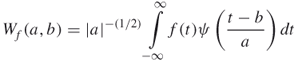
where ![]() is the position and
is the position and ![]() is the scale. The scale
is the scale. The scale ![]() in wavelet transform means the
in wavelet transform means the ![]() th resolution of the data. Taking
th resolution of the data. Taking ![]() and
and ![]() , we get the wavelet spectrum as
, we get the wavelet spectrum as
![]()
where ![]() .
.
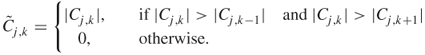
For simplicity, the scale ![]() can be selected as
can be selected as ![]() , which are more adjacent and can be used to capture more details of the data. The wavelet spectrum is calculated by summing the squares of the coefficients in each scale
, which are more adjacent and can be used to capture more details of the data. The wavelet spectrum is calculated by summing the squares of the coefficients in each scale ![]() . The local wavelet spectrum is defined through the modulus maxima of the coefficients [67] as
. The local wavelet spectrum is defined through the modulus maxima of the coefficients [67] as ![]() , where
, where
The maximum of the wavelet spectrum and the maximum of the local wavelet spectrum were applied in the prediction of structural classes and families of proteins [53].
In our work, we chose the Daubechies wavelet, which is commonly used as a signal processing tool. These wavelet functions are compactly supported wavelets with extremal phase and highest number of vanishing moments for a given support width. They are orthogonal and biorthogonal functions. The Daubechies wavelets can improve the frequency domain characteristics of other wavelets [19].
16.2.11 Recurrence Quantification Analysis
The recurrence plot (RP) is a purely graphical tool originally proposed by Eckmann et al. [21] to detect patterns of recurrence in the data. For a time series ![]() with length
with length ![]() , we can embed it into the space
, we can embed it into the space ![]() with embedding dimension
with embedding dimension ![]() and a time delay
and a time delay ![]() . We write
. We write ![]()
![]() , where
, where ![]() . In this way we obtain
. In this way we obtain ![]() vectors (points) in the embedding space
vectors (points) in the embedding space ![]() . We gave some numerical explanations for the selection of
. We gave some numerical explanations for the selection of ![]() and
and ![]() in our earlier paper [52].
in our earlier paper [52].
From the ![]() points, we can calculate the distance matrix (DM), which is a square
points, we can calculate the distance matrix (DM), which is a square ![]() matrix. The elements of DM are the distances between all possible combinations of
matrix. The elements of DM are the distances between all possible combinations of ![]() points and
points and ![]() points. They are computed according to the norming function selected. Generally, the Euclidean norm is used [47]. DM can be rescaled by dividing each element in the DM by a certain value as this allows systems operating on different scales to be statistically compared. For such a value, the maximum distance of the entire matrix DM is the most commonly used (and recommended) rescaling option, which redefines the DM over the unit interval (0.0–100.0%).
points. They are computed according to the norming function selected. Generally, the Euclidean norm is used [47]. DM can be rescaled by dividing each element in the DM by a certain value as this allows systems operating on different scales to be statistically compared. For such a value, the maximum distance of the entire matrix DM is the most commonly used (and recommended) rescaling option, which redefines the DM over the unit interval (0.0–100.0%).
Once the rescaled DM = ![]() is calculated, it can be transformed into a recurrence matrix (RM) of distance elements within a threshold
is calculated, it can be transformed into a recurrence matrix (RM) of distance elements within a threshold ![]() (namely, radius). RM =
(namely, radius). RM = ![]() and
and ![]() where
where ![]() is the Heaviside function
is the Heaviside function
16.26 
RP is simply a visualization of RM by plotting the points on the ![]() plane for those elements in RM with values equal to 1. If
plane for those elements in RM with values equal to 1. If ![]() , we say that
, we say that ![]() points recur with reference to
points recur with reference to ![]() points. For any
points. For any ![]() , since
, since ![]() , the RP has always a black main diagonal line. Furthermore, the RP is symmetric with respect to the main diagonal as
, the RP has always a black main diagonal line. Furthermore, the RP is symmetric with respect to the main diagonal as ![]() .
. ![]() is a crucial parameter of RP. If
is a crucial parameter of RP. If ![]() is chosen too small, there may be almost no recurrence points and we will not be able to learn about the recurrence structure of the underlying system. On the other hand, if
is chosen too small, there may be almost no recurrence points and we will not be able to learn about the recurrence structure of the underlying system. On the other hand, if ![]() is chosen too large, almost every point is a neighbor of every other point, which leads to a large number of artifacts [68]. Selection of
is chosen too large, almost every point is a neighbor of every other point, which leads to a large number of artifacts [68]. Selection of ![]() was discussed numerically in [52].
was discussed numerically in [52].
Recurrence quantification analysis (RQA) is a relatively new nonlinear technique proposed by Zbilut and Webber [22, 23] that can quantify the information supplied by RP. Eight recurrence variables are usually used to quantify RP [68]. It should be pointed out that the recurrence points in the following definitions consist only of those in the upper triangle in RP (excluding the main diagonal line). The first recurrence variable is %recurrence (%REC). %REC is ameasure of the density of recurrence points in the RP. This variable can range from 0% (no recurrent points) to 100% (all points are recurrent). The second recurrence variable is %determinism (%DET). %DET measures the proportion of recurrent points forming diagonal line structures. For this variable, we have to first decide at least how many adjacent recurrent points are needed to define a diagonal line segment. Obviously, the minimum number required (and commonly used) is 2. The third recurrence variable is linemax (![]() ), which is simply the length of the longest diagonal line segment in RP. This is a very important recurrence variable because it inversely scales with the largest positive Lyapunov exponent. The fourth recurrence variable is entropy (ENT), which is the Shannon information entropy of the distribution probability of the length of the diagonal lines. The fifth recurrence variable is trend (TND), which quantifies the degree of system stationarity. It is calculated as the slope of the least squares regression of %local recurrence as a function of the displacement from the main diagonal. It should be made clear that the so called %local recurrence is in fact the proportion of recurrent points on certain line parallel to the main diagonal over the length of this line. %recurrence is calculated on the whole upper triangle in RP while %local recurrence is computed on only certain lines in RP, so it is termed as local. Multiplying by 1000 increases the gain of the TND variable. The remaining three variables are defined on the basis of the vertical line structure. The sixth recurrence variable is %laminarity ( %LAM). %LAM is analogous to %DET but is calculated with recurrent points constituting vertical line structures. Similarly, we also select 2 as the minimum number of adjacent recurrent points to form a vertical line segment. The seventh variable, trapping time (TT), is the average length of vertical line structures. The eighth recurrence variable is maximal length of the vertical lines in RP (
), which is simply the length of the longest diagonal line segment in RP. This is a very important recurrence variable because it inversely scales with the largest positive Lyapunov exponent. The fourth recurrence variable is entropy (ENT), which is the Shannon information entropy of the distribution probability of the length of the diagonal lines. The fifth recurrence variable is trend (TND), which quantifies the degree of system stationarity. It is calculated as the slope of the least squares regression of %local recurrence as a function of the displacement from the main diagonal. It should be made clear that the so called %local recurrence is in fact the proportion of recurrent points on certain line parallel to the main diagonal over the length of this line. %recurrence is calculated on the whole upper triangle in RP while %local recurrence is computed on only certain lines in RP, so it is termed as local. Multiplying by 1000 increases the gain of the TND variable. The remaining three variables are defined on the basis of the vertical line structure. The sixth recurrence variable is %laminarity ( %LAM). %LAM is analogous to %DET but is calculated with recurrent points constituting vertical line structures. Similarly, we also select 2 as the minimum number of adjacent recurrent points to form a vertical line segment. The seventh variable, trapping time (TT), is the average length of vertical line structures. The eighth recurrence variable is maximal length of the vertical lines in RP (![]() ), which is similar to
), which is similar to ![]() .
.
16.2.12 Empirical Mode Decomposition and Similarity of Proteins
Empirical mode decomposition (EMD) was originally designed for non-linear and nonstationary data analysis by Huang et al. [24]. The traditional EMD decomposes a time series into components called intrinsic mode functions (IMFs) to define meaningful frequencies of a signal.
Lin et al. [25] proposed a new algorithm for EMD. Instead of using the envelopes generated by spline, a lowpass filter is used to generate a moving average to replace the mean of the envelopes. The essence of the shifting algorithm remains. Let ![]() be a lowpass filter operator, for which
be a lowpass filter operator, for which ![]() represents a moving average of
represents a moving average of ![]() . We now define
. We now define ![]() . In this approach, the lowpass filter
. In this approach, the lowpass filter ![]() is dependent on the data
is dependent on the data ![]() . For a given
. For a given ![]() , we choose a lowpass filter
, we choose a lowpass filter ![]() accordingly and set
accordingly and set ![]() , where
, where ![]() is the identity operator. The first IMF in the new EMD is given by
is the identity operator. The first IMF in the new EMD is given by ![]() , and subsequently the
, and subsequently the ![]() th IMF
th IMF ![]() is obtained first by selecting a lowpass filter
is obtained first by selecting a lowpass filter ![]() according to the data
according to the data ![]() and iterations
and iterations ![]() , where
, where ![]() . The process stops when
. The process stops when ![]() has at most one local maximum or local minimum. Lin et al. [25] suggested using the filter
has at most one local maximum or local minimum. Lin et al. [25] suggested using the filter ![]() given by
given by ![]() . We selected the mask
. We selected the mask
![]()
in our work [53].
Let ![]() . The original signal can be expressed as
. The original signal can be expressed as ![]() , where the number
, where the number ![]() can be chosen according to a standard deviation. In our work, the number of components in IMFs was set as 4 due to the short length of some amino acid sequences [53].
can be chosen according to a standard deviation. In our work, the number of components in IMFs was set as 4 due to the short length of some amino acid sequences [53].
The similarity value of two proteins at each component (IMF) is obtained as the maximum absolute value of the correlation coefficient. In our work [53], a new cross-correlation coefficient ![]() is defined by
is defined by
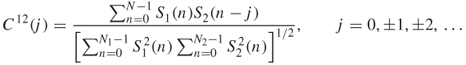
where ![]() is the length of the intersection of two signals with lag
is the length of the intersection of two signals with lag ![]() ,
, ![]() is the length of signal
is the length of signal ![]() , and
, and ![]() is the length of signal
is the length of signal ![]() . The maximum absolute value C of all the correlation coefficients of the components is considered as the similarity value for two proteins.
. The maximum absolute value C of all the correlation coefficients of the components is considered as the similarity value for two proteins.
16.3 Results and conclusions
In our earlier paper [50], we selected the amino acid sequences of 43 large proteins from the RCSB Protein Data Bank (http://www.rcsb.org/pdb/index.html). These 43 proteins belong to four structural classes according to their secondary structures:
In a parameter space, one point represents a protein. We wanted to determine whether the proteins can be separated from four structural classifications in these parameter spaces. We found that we can propose a method which consists of three components to cluster proteins [50]. We used Fisher's linear discriminant algorithm to give a quantitative assessment of our clustering on the selected proteins. The discriminant accuracies are satisfactory. In particular, they reach 94.12% and 88.89% in separating ![]() proteins from
proteins from ![]() proteins in a 3D space.
proteins in a 3D space.
We [51], considered a set of 49 large proteins that included the 43 proteins studied earlier [50]. Given an amino acid sequence of one protein, we first converted it into its measure representation ![]() based on the six-letter model with length
based on the six-letter model with length ![]() . Then we calculated
. Then we calculated ![]() , and
, and ![]() for the measures
for the measures ![]() of the 49 selected proteins. We then converted the amino acid sequences of proteins into their RSWH sequences according to the revised Schneider–Wrede hydrophobicity scale. We used such sequences to construct the measures
of the 49 selected proteins. We then converted the amino acid sequences of proteins into their RSWH sequences according to the revised Schneider–Wrede hydrophobicity scale. We used such sequences to construct the measures ![]() . The ordinary multifractal analysis was then performed on these measures. The AMFA was also performed on the RSWH sequences. Then nine parameters from these analyses were selected as candidates for constructing parameter spaces. We proposed another three steps to cluster protein structures [51]. Fisher's linear discriminant algorithm was used to assess our clustering accuracy on the 49 selected large proteins. The discriminant accuracies are satisfactory. In particular, they reach
. The ordinary multifractal analysis was then performed on these measures. The AMFA was also performed on the RSWH sequences. Then nine parameters from these analyses were selected as candidates for constructing parameter spaces. We proposed another three steps to cluster protein structures [51]. Fisher's linear discriminant algorithm was used to assess our clustering accuracy on the 49 selected large proteins. The discriminant accuracies are satisfactory. In particular, they reach ![]() and
and ![]() in separating the
in separating the ![]() proteins from the
proteins from the ![]() proteins in a parameter space;
proteins in a parameter space; ![]() and
and ![]() , in separating the
, in separating the ![]() proteins from the
proteins from the ![]() proteins in another parameter space; and
proteins in another parameter space; and ![]() and
and ![]() , in separating the
, in separating the ![]() proteins from the
proteins from the ![]() proteins in the last parameter space.
proteins in the last parameter space.
We [52], intended to predict protein structural classes (![]() ,
, ![]() ,
, ![]() , or
, or ![]() ) for low-similarity datasets. Two datasets were used widely: 1189 (containing 1092 proteins) and 25PDB (containing 1673 proteins) with sequence similarity values of 40% and 25%, respectively. We proposed decomposing the chaos game representation of proteins into two kinds of time series. Then we applied recurrence quantification analysis to analyze these time series. For a given protein sequence, a total of 16 characteristic parameters can be calculated with RQA, which are treated as feature representations of the protein. On the basis of such feature representation, the structural class for each protein was predicted with Fisher's linear discriminant algorithm. The overall accuracies with step-by-step procedure are 65.8% and 64.2% for 1189 and 25PDB datasets, respectively. With one-against-others procedure used widely, we compared our method with five other existing methods. In particular, the overall accuracies of our method are 6.3% and 4.1% higher for the two datasets, respectively. Furthermore, only 16 parameters were used in our method, which is less than that used by other methods.
) for low-similarity datasets. Two datasets were used widely: 1189 (containing 1092 proteins) and 25PDB (containing 1673 proteins) with sequence similarity values of 40% and 25%, respectively. We proposed decomposing the chaos game representation of proteins into two kinds of time series. Then we applied recurrence quantification analysis to analyze these time series. For a given protein sequence, a total of 16 characteristic parameters can be calculated with RQA, which are treated as feature representations of the protein. On the basis of such feature representation, the structural class for each protein was predicted with Fisher's linear discriminant algorithm. The overall accuracies with step-by-step procedure are 65.8% and 64.2% for 1189 and 25PDB datasets, respectively. With one-against-others procedure used widely, we compared our method with five other existing methods. In particular, the overall accuracies of our method are 6.3% and 4.1% higher for the two datasets, respectively. Furthermore, only 16 parameters were used in our method, which is less than that used by other methods.
Family identification is helpful in predicting protein functions. Since most protein sequences are relatively short, we first randomly linked the protein sequences from the same family or superfamily together to form 120 longer protein sequences [53], and each structural class contains 30 linked protein sequences. Then we used, the 6-letter model, 12-letter model, 20-letter model, the revised Schneider–Wrede scale hydrophobicity, solvent accessibility, and stochastic standard state accessibility values to convert linked protein sequences to numerical sequences. Then we calculated the generalized fractal dimensions ![]() , the related spectra
, the related spectra ![]() , the multifractal spectra
, the multifractal spectra ![]() , and the
, and the ![]() curves of the six kinds of numerical sequences of all 120 linked proteins. The curves of
curves of the six kinds of numerical sequences of all 120 linked proteins. The curves of ![]() ,
, ![]() showed that the numerical sequences from linked proteins are multifractal-like and sufficiently smooth. The
showed that the numerical sequences from linked proteins are multifractal-like and sufficiently smooth. The ![]() curves resemble the phase transition at a certain point, while the
curves resemble the phase transition at a certain point, while the ![]() and
and ![]() curves indicate the multifractal scaling features of proteins. In wavelet analysis, the choice of a wavelet function should be carefully considered. Different wavelet functions represent a given function with different approximation components. We [53], chose the commonly used Daubechies wavelet db2 and computed the maximum of the wavelet spectrum and the maximum of the local wavelet spectrum for the six kinds of numerical sequences of all 120 linked proteins. The parameters from the multifractal and wavelet analyses were used to construct parameter spaces where each linked protein is represented by a point. The four classes of proteins were then distinguished in these parameter spaces. The discriminant accuracies obtained through Fisher's linear discriminant algorithm are satisfactory in separating these classes. We found that the linked proteins from the same family or superfamily tend to group together and can be separated from other linked proteins. The methods are also helpful to identify the family of an unknown protein.
curves indicate the multifractal scaling features of proteins. In wavelet analysis, the choice of a wavelet function should be carefully considered. Different wavelet functions represent a given function with different approximation components. We [53], chose the commonly used Daubechies wavelet db2 and computed the maximum of the wavelet spectrum and the maximum of the local wavelet spectrum for the six kinds of numerical sequences of all 120 linked proteins. The parameters from the multifractal and wavelet analyses were used to construct parameter spaces where each linked protein is represented by a point. The four classes of proteins were then distinguished in these parameter spaces. The discriminant accuracies obtained through Fisher's linear discriminant algorithm are satisfactory in separating these classes. We found that the linked proteins from the same family or superfamily tend to group together and can be separated from other linked proteins. The methods are also helpful to identify the family of an unknown protein.
Zhu et al. [54] applied component similarity analysis based on EMD and the new cross-correlation coefficient formula (16.27) to protein pairs. They then considered maximum absolute value ![]() of all the correlation coefficients of the components as the similarity value for two proteins. They also created the threshold of correlation [54]. Two signals are considered strongly correlated if the correlation coefficient exceeds
of all the correlation coefficients of the components as the similarity value for two proteins. They also created the threshold of correlation [54]. Two signals are considered strongly correlated if the correlation coefficient exceeds ![]() and weakly correlated if the coefficient is between
and weakly correlated if the coefficient is between ![]() and
and ![]() . The results showed that the functional relationships of some proteins may be revealed by component analysis of their IMFs. Compared with those traditional alignment methods, component analysis can be evaluated and described easily. It illustrates that EMD and component analysis can complement traditional sequence similarity approaches that focus on the alignment of amino acids.
. The results showed that the functional relationships of some proteins may be revealed by component analysis of their IMFs. Compared with those traditional alignment methods, component analysis can be evaluated and described easily. It illustrates that EMD and component analysis can complement traditional sequence similarity approaches that focus on the alignment of amino acids.
From our analyses, we found that the measure representation based on the detailed HP model and six-letter model, time series representation based on physicochemical features of amino acids, ![]() -curve representation, the chaos game representation of proteins can provide much information for predicting structure classes and functions of proteins. Fractal methods are useful to analyze protein sequences. Our methods may play a complementary role in the existing methods.
-curve representation, the chaos game representation of proteins can provide much information for predicting structure classes and functions of proteins. Fractal methods are useful to analyze protein sequences. Our methods may play a complementary role in the existing methods.
Acknowledgment
This work was supported by the Natural Science Foundation of China (Grant 11071282); the Chinese Program for Changjiang Scholars and Innovative Research Team in University (PCSIRT) (Grant No. IRT1179); the Research Foundation of Education Commission of Hunan Province, China (Grant 11A122); the Lotus Scholars Program of Hunan Province of China; the Aid program for Science and Technology Innovative Research Team in Higher Educational Institutions of Hunan Province of China; and the Australian Research Council (Grant DP0559807).
References
1. Hou J, Jun S-R, Zhang C, Kim S-H, Global mapping of the protein structure space and application in structure-based inference of protein function, Natl. Acad. Sci. USA 102:3651–3656 (2005).
2. Anfinsen C, Principles that govern the folding of protein chains, Science 181:223–230 (1973).
3. Chothia C, One thousand families for the molecular biologists, Nature (Lond.) 357:543–544 (1992).
4. Frishman D, Argos P, Knowledge-based protein secondary structure assignment, Proteins 23:566–579 (1995).
5. Crooks GE, Brenner SE, Protein secondary structure: Entropy, correlation and prediction, Bioinformatics 20:1603–1611 (2004).
6. Adamczak R, Porollo A, Meller J, Combining prediction of secondary structure and solvent accessibility in proteins, Proteins 59:467–475 (2005).
7. Levitt M, Chothia C, Structural patterns in globular proteins, Nature 261:552–558 (1976).
8. Service., A dearth of new folds, Science 307:1555–1555 (2005).
9. Chou KC, Progress in protein structural class prediction and its impact to bioinformatics and proteomics, Curr. Protein Peptide Sci. 6(5):423–436 (2005).
10. Trad CH, Fang Q, Cosic I, Protein sequence comparison based on the wavelet transform approach, Protein Eng. 15(3):193–203 (2002).
11. Lesk AM, Computational Molecular Biology: Sources and Methods for Sequence Analysis, Oxford Univ. Press, 1988.
12. Mandelbrot BB, The Fractal Geometry of Nature, Academic Press, New York, 1983.
13. Feder J, Fractals, Plenum Press, New York, 1988.
14. Grassberger P, Procaccia I, Characterization of strange attractors, Rev. Lett. 50:346–349 (1983).
15. Yu ZG, Anh V, Eastes R, Multifractal analysis of geomagnetic storm and solar flare indices and their class dependence, J. Geophys. Res. 114:A05214 (2009).
16. Yu ZG, Anh VV, Lau KS, Measure representation and multifractal analysis of complete genome, Phys. Rev. E 64:031903 (2001).
17. Yu ZG, Anh VV, Wang B, Correlation property of length sequences based on global structure of complete genome, Phys. Rev. E 63:011903 (2001).
18. Peng CK, Buldyrev S, Goldberg AL, Havlin S, Sciortino F, Simons M, Stanley HE, Long-range correlations in nucleotide sequences, Nature 356:168–170 (1992).
19. Chui CK, An Introduction to Wavelets, Academic Press Professional, San Diego, 1992.
20. Daubechies I, Ten Lectures on Wavelets, SIAM, Philadelphia, 1992.
21. Eckmann JP, Kamphorst SO, Ruelle D, Recurrence plots of dynamical systems, Europhys. Lett. 4:973–977 (1987).
22. Zbilut JP, Webber CL Jr, Embeddings and delays as derived from quantification of recurrence plots, Phys. Lett. A 171:199–203 (1992).
23. Webber CL Jr, Zbilut JP, Dynamical assessment of physiological systems and states using recurrence plot strategies, J. Appl. Physiol. 76:965–973 (1994).
24. Huang N, Shen Z, Long SR, Wu ML, Shih HH, Zheng Q, Yen NC, Tung CC, Liu HH, The empirical mode decomposition and Hilbert spectrum for nonlinear and nonstationary time series analysis, Proc. Roy. Soc. Lond. A 454:903–995 (1998).
25. Lin L, Wang Y, Zhou H, Iterative filtering as an alternative for empirical mode decomposition, Adv. Adapt. Data Anal. 1(4):543–560 (2009).
26. Janosi IM, Muller R, Empirical mode decomposition and correlation properties of long daily ozone records, Phys. Rev. E 71:056126 (2005).
27. ZG Yu, Anh V, Wang Y, Mao D, Wanliss J, Modeling and simulation of the horizontal component of the geomagnetic field by fractional stochastic differential equations in conjunction with empirical mode decomposition, J. Geophys. Res. 115:A10219 (2010).
28. Dewey TG, Fractal analysis of proton-exchange kinetics in lysozyme, Proc. Natl. Acad. Sci. USA 91:12101–12104 (1994).
29. Fiser A, Tusnady GE, Simon I, Chaos game representation of protein structure, J. Mol. Graphies 12:302–304 (1994).
30. Yu ZG, Anh VV, Lau KS, Fractal analysis of large proteins based on the detailed HP model, Physica A 337:171–184 (2004).
31. Yu ZG, Anh VV, Lau KS, Chaos game representation, and multifractal and correlation analysis of protein sequences from complete genome based on detailed HP model, J. Theor. Biol. 226:341–348 (2004).
32. Enright MB, Leitner DM, Mass fractal dimension and the compactness of proteins, Phys. Rev. E 71:011912 (2005).
33. Moret MA, Miranda JGV, Nogueira E, et al, Self-similarity and protein chains, Phys. Rev. E 71:012901 (2005).
34. Pavan YS, Mitra CK, Fractal studies on the protein secondary structure elements, Indian J. Biochem. Biophys. 42:141–144 (2005).
35. Balafas JS, Dewey TG, Multifractal analysis of solvent accessibilities in proteins, Phys. Rev. E 52:880–887 (1995).
36. Yu ZG, Anh VV, Lau KS, Multifractal and correlation analysis of protein sequences from complete genome, Phys. Rev. E 68:021913 (2003).
37. Mandell AJ, Selz KA, Shlesinger MF, Mode maches and their locations in the hydrophobic free energy sequences of peptide ligands and their receptor eigenfunctions, Proc. Natl. Acad. Sci. USA 94:13576–13581 (1997).
38. Mandell AJ, Selz KA, Shlesinger MF, Wavelet transfermation of protein hydrophobicity sequences suggests their memberships in structural families, Physica A 244:254–262 (1997).
39. Selz KA, Mandell AJ, Shlesinger MF, Hydrophobic free energy eigenfunctions of pore, channel, and transporter proteins contain β-burst patterns, Biophys. J. 75:2332–2342 (1998).
40. Hirakawa H, Muta S, Kuhara S, The hydrophobic cores of proteins predicted by wavelet analysis, Bioinformatics 15:141–148 (1999).
41. Chen H, Gu F, Liu F, Predicting protein secondary structure using continuous wavelet transform and Chou–Fasman method, Proc. 27th Annual IEEE, Engineering in Medicine and Biology Conf. 2005.
42. Marsolo K, Ramamohanarao K, Structure-based on querying of proteins using wavelets, Proc.15th Int. ACM Conf. Information and Knowledge Management, 2006, pp. 24–33.
43. Qiu JD, Liang RP, Zou XY, Mo JY, Prediction of protein secondary structure based on continuous wavelet transform, Talanta 61(3):285–293 (2003).
44. Rezaei M, Abdolmaleki P, Jahandideh S, Karami Z, Asadabadi EB, Sherafat MA, Abrishami-Moghaddam H, Fadaie M, Foroozan M, Prediction of membrane protein types by means of wavelet analysis and cascaded neural networks, J. Theor. Biol. 254(4):817–820 (2008).
45. Pando J, Sands L, Shaheen SE, Detection of protein secondary structures via the discrete wavelet transform, Phys. Rev. E 80:051909 (2009).
46. Webber CL Jr, Giuliani A, Zbilut JP, Colosimo A, Elucidating protein secondary structures using alpha-carbon recurrence quantifications, Proteins: Struct., Funct., Genet. 44:292–303 (2001).
47. Giuliani A, Benigni R, Zbilut JP, Webber CL Jr., Sirabella P, Colosimo A, Signal analysis methods in elucidation of protein sequence-structure relationships, Chem. Rev. 102:1471–1491 (2002).
48. Shi F, Chen Q, Niu X, Functional similarity analyzing of protein sequences with empirical mode decomposition, Proc. 4th Int. Conf. Fuzzy Systems and Knowledge Discovery, 2007.
49. Shi F, Chen QJ, Li NN, Hilbert Huang transform for predicting proteins subcellular location, J. Biomed. Sci. Eng. 1:59–63 (2008).
50. Yu ZG, Anh VV, Lau KS, Zhou LQ, Fractal and multifractal analysis of hydrophobic free energies and solvent accessibilities in proteins, Phys. Rev. E. 73:031920 (2006).
51. Yang JY, Yu ZG, Anh V, Clustering structure of large proteins using multifractal analyses based on 6-letters model and hydrophobicity scale of amino acids, Chaos, Solitons, Fractals 40:607–620 (2009).
52. Yang JY, Peng ZL, Yu ZG, Zhang RJ, Anh V, Wang D, Prediction of protein structural classes by recurrence quantification analysis based on chaos game representation, J. Theor. Biol. 257:618–626 (2009).
53. Zhu SM, Yu ZG, Anh V, Protein structural classification and family identification by multifractal analysis and wavelet spectrum, Chin. Phys. B 20:010505 (2011).
54. Zhu SM, Yu ZG, Anh V, Yang SY, Analysing the similarity of proteins based on a new approach to empirical mode decomposition, Proc. 4th Int. Conf. Bioinformatics and Biomedical Engineering (ICBBE2010), vol. 1, (2010).
55. Chou PY, Fasman GD, Prediction of protein conformation, Biochemistry 13:222–245 (1974).
56. Bordo D, Argos P, Suggestions for safe residue substitutions in site-directed mutagenesis, J. Mol. Biol. 217:721–729 (1991).
57. Rose GD, Geselowitz AR, Lesser GJ, Lee RH, Zehfus MH, Hydrophobicity of amino acid residues in globular proteins, Science 229:834–838 (1985).
58. Krigbaum WR, Komoriya A, Local interactions as a structure determinant for protein molecules: II, Biochim. Biophys. Acta 576:204–228 (1979).
59. Zhang R, Zhang CT, Z curves, an intuitive tool for visualizing and analyzing the DNA sequences, J. Biomol. Struct. Dyn. 11:767–782 (1994).
60. Basu S, Pan A, Dutta C, Das J, Chaos game representation of proteins, J. Mol. Graphics 15:279–289 (1997).
61. Deschavanne P, Tufféry P, Exploring an alignment free approach for protein classification and structural class prediction, Biochimie 90:615–625 (2008).
62. Jeffrey HJ, Chaos game representation of gene structure, Nucleic Acids Res, 18:2163–2170 (1990).
63. Brown TA, Genetics, 3rd ed., Chapman & Hall, London, 1998.
64. Barnsley MF, Demko S, Iterated function systems and the global construction of fractals, Proc. Roy. Soc. (Lond.) 399:243–275 (1985).
65. Vrscay ER, Iterated function systems: Theory, applications and the inverse problem, in Belair J, Dubuc S. (eds.), Fractal Geometry and Analysis, NATO ASI series, Kluwer, 1991.
66. Canessa E, Multifractality in time series, J. Phys. A: Math. Genet. 33:3637–3651 (2000).
67. Arneodo A, Bacry E, Muzy JF, The thermodynamics of fractals revisited with wavelets, Physica A 213:232–275 (1995).
68. Marwan N, Romano MC, Thiel M, Kurths J, Recurrence plots for the analysis of complex systems, Phys. Reports 438:237–329 (2007).