
Chapter 18
Network Algorithms For Protein Interactions
18.1 Introduction
Graphs or networks are a fundamental way of representing connections between objects or concepts. Connections between proteins can identify functional groups of proteins, and how various proteins work together. Studies of the function of proteins are fundamental in current biological research [40]. We have been able to sequence entire genomes and can identify large numbers of individual genes. However, while the syntax of the genes is rapidly becoming clearer, the semantics or meaning of those genes is still mostly shrouded in mystery. This mystery has deepened in recent years as it has become apparent hat there is no one-to-one connection between genes and the proteins that actually perform functions in organisms.
In order to unlock the information about how proteins carry out their function, we first need to understand which proteins work together. High-throughput experiments have been able to create interaction networks for large numbers of proteins. One particular method is tandem affinity purification (TAP), which was developed in the late 1990s [31], and has been used to obtain large-scale interaction networks. For example, a large-scale protein–protein interaction (PPI) network was constructed for baker's yeast (Saccharomyces cerevisiae) [21] using TAP combined with mass spectrometry to identify the proteins in the complexes. The study [21] identified 7123 interactions among a set of 2708 proteins. Note that this makes the network of interaction quite sparse: only 7123 interactions are identified out of a maximum of ![]() possible interactions.
possible interactions.
The task that is considered in this chapter is to cluster the set of proteins into natural groups that operate together. These groups should be functional groups and can often be identified as serving a particular purpose in the life of a cell [37].
From the data mining perspective, numerous issues arise in dealing with these PPI networks. Many datasets have numeric values for a number of attributes of each data item (such as the well-known “iris” dataset of Fisher) from which measures similarity or nearness are computed. In PPI networks, on the other hand, the data are given directly in the form of a network. A second issue is that with biological systems and large-scale experiments, a relatively high error rate is expected. Since the PPI network is fairly sparse, even if the error rate is kept reasonably low, the number of false positives is likely to be at least a significant percentage of the identified interactions. Oliveira and Seok [24, 27, 28] have addressed these issues.
In this chapter we look at algorithms for clustering that use optimization methods, often combined with hierarchical methods, as exemplified by the author's work [24, 27–29] and the work of others, [e.g., [40]].
18.2 Optimization approaches to clustering
Anyone can cluster a dataset. Simply split the items wherever you please, and you have a cluster. The problem is that the clusters so created are unlikely to have any significant coherence. What we really need are high-quality clusters. If we can define the quality of a cluster, then the problem of clustering becomes an optimization problem.
18.2.1 Similarities and Distances
The basic data needed for a clustering then are a measure of the similarity between two data items. Since data items themselves may be given as vectors of numbers or as a collection of attributes, the usual first step is to define the similarity between two data items by a function of the entries or attributes of the data items. If the data items are given as vectors of numbers where the ![]() th entry is the strength of a certain attribute, then we can represent the similarity in terms of the distance between the two vectors in a certain norm; for data items
th entry is the strength of a certain attribute, then we can represent the similarity in terms of the distance between the two vectors in a certain norm; for data items ![]() and
and ![]() represented by vectors
represented by vectors ![]() and
and ![]() , we take the distance between them to be
, we take the distance between them to be ![]() , where
, where ![]() is a measure of the size of
is a measure of the size of ![]() . The most common norm is the Euclidean norm, which is given by
. The most common norm is the Euclidean norm, which is given by ![]() . Other norms include the Manhattan matrix or 1-norm:
. Other norms include the Manhattan matrix or 1-norm: ![]() , and the max-norm or
, and the max-norm or ![]() -norm:
-norm: ![]() . Norms have a number of basic properties:
. Norms have a number of basic properties:
 , and if
  is possible only if
  .
. for any scale factor
  .
. for any
  and
and  ; this is called the triangle inequality.
For clustering applications it is important that the different components of the data vectors ![]() be scaled similarly. If, for example, the
be scaled similarly. If, for example, the ![]() th component of the
th component of the ![]() vectors is scaled to be much larger than the other components of
vectors is scaled to be much larger than the other components of![]() , then the distance measurement will mainly reflect differences in that component.
, then the distance measurement will mainly reflect differences in that component.
Often it is better to think of weights or dissimilarities instead of distances. For example, we could take ![]() , which may be more appropriate; doubling the distance quadruples the weight in this example. This might be appropriate where outliers should be removed from clusters, but not appropriate where a chain of connections might connect apparently distant data items.
, which may be more appropriate; doubling the distance quadruples the weight in this example. This might be appropriate where outliers should be removed from clusters, but not appropriate where a chain of connections might connect apparently distant data items.
The values ![]() represent dissimilatiries, and the greater the dissimilarity, the less similar the data items are. If we need to obtain similarities, we will treat then as functions of the distances:
represent dissimilatiries, and the greater the dissimilarity, the less similar the data items are. If we need to obtain similarities, we will treat then as functions of the distances: ![]() is the similarity between data item
is the similarity between data item ![]() and data item
and data item ![]() . The function
. The function ![]() should be a decreasing function of the distance; after all, the greater the distance, the less similar. We will assume that similarity, like distance, must be a nonnegative quantity.
should be a decreasing function of the distance; after all, the greater the distance, the less similar. We will assume that similarity, like distance, must be a nonnegative quantity.
A desirable property of the collection of weights ![]() or similarities
or similarities ![]() is that the array of these values
is that the array of these values ![]() or
or ![]() should be data-sparse; that is, the arrays should be representable in some way by many fewer than the
should be data-sparse; that is, the arrays should be representable in some way by many fewer than the ![]() entries that appear in the arrays. This is perhaps easier to do with the matrix of similarities if we set
entries that appear in the arrays. This is perhaps easier to do with the matrix of similarities if we set ![]() so that
so that ![]() results in zero similarity. This can result in a sparse matrix (one in which all but a small fraction of the
results in zero similarity. This can result in a sparse matrix (one in which all but a small fraction of the ![]() entries are zero) if
entries are zero) if ![]() is suitably chosen. This can be a reasonable approach, as the degree of similarity between data items is usually important only if the data items are close. Sparse matrices can be stored and used for computation in a memory-efficient way by storing only the nonzero entries along with some additional data structures to navigate the sparsity structure [38]. If the matrix of distances is needed, then the values
is suitably chosen. This can be a reasonable approach, as the degree of similarity between data items is usually important only if the data items are close. Sparse matrices can be stored and used for computation in a memory-efficient way by storing only the nonzero entries along with some additional data structures to navigate the sparsity structure [38]. If the matrix of distances is needed, then the values ![]() can also be stored in a data-sparse manner, perhaps by storing
can also be stored in a data-sparse manner, perhaps by storing ![]() as a sparse matrix.
as a sparse matrix.
18.2.2 Objective Functions
However, to measure the similarities or dissimilarities between data items, we need a way of measuring the quality of the clustering. We will focus on just a few objective functions; there is considerable variation in the objective functions that can be used for this task. In general, there are two objective functions:
Phrased in this way, the problem is a multiobjective optimization problem [7]. As with most multiobjective optimization problems, there is strong tension between the two objectives; the clustering that has the highest coherence within clusters is the clustering in which each data item forms its own cluster, andmaximizing distance between different clusters tends to result in few clusters, or perhaps just one. The theory of multiobjective optimization has a conceptual remedy to this tension between objectives, which is the concept of Pareto optima; a Pareto optima is a solution where an improvement in one objective can only be made by worsening another objective. There is typically a large set of Pareto optima. The user or application decides how the tradeoff between the objectives should be carried out.
In practice, a multiobjective problem is replaced by a single-objective function that in some way captures the competing objectives. The tradeoff is built into this objective. Often we can incorporate weights or other parameters that allow us to modify the tradeoff between the objectives.
The first objective function that we will consider is a well-known objective for graph bisection: splitting a graph ![]() with weighted edges into two disjoint sets of vertices
with weighted edges into two disjoint sets of vertices ![]() and
and ![]() where
where ![]() . The objective to be minimized is the sum of weights of edges connecting
. The objective to be minimized is the sum of weights of edges connecting ![]() and
and ![]() :
:
Minimizing this objective without any further constraints leads to either ![]() and
and ![]() , or
, or ![]() and
and ![]() , both with
, both with ![]() . Clearly this is not a very useful result. However, if we add the constraint that the number of vertices in
. Clearly this is not a very useful result. However, if we add the constraint that the number of vertices in ![]() and in
and in ![]() are at least similar in magnitude, the problem becomes much more interesting. For applications in parallel computing, if
are at least similar in magnitude, the problem becomes much more interesting. For applications in parallel computing, if ![]() and
and ![]() represent the tasks to be completed and the edge weights represent the communication needed between the associated tasks, then
represent the tasks to be completed and the edge weights represent the communication needed between the associated tasks, then ![]() represents the communication needed between a pair of processors with tasks in
represents the communication needed between a pair of processors with tasks in ![]() executed on processor 1, and
executed on processor 1, and ![]() the tasks executed on processor 2. Minimizing
the tasks executed on processor 2. Minimizing ![]() corresponds to minimizing interprocessor communication. However, in the parallel computing application, it is also important to balance the load between the processors. The standard balance condition is that the number of vertices in
corresponds to minimizing interprocessor communication. However, in the parallel computing application, it is also important to balance the load between the processors. The standard balance condition is that the number of vertices in ![]() (denoted
(denoted ![]() ) differs from the number of vertices in
) differs from the number of vertices in ![]() (
(![]() ) by no more than one:
) by no more than one:
This optimization problem can be put into matrix–vector form by creating a decision variable or vector ![]() with
with ![]() components where
components where ![]() if
if ![]() and
and ![]() if
if ![]() . Then the objective and constraints can be represented by the following integer optimization (or integer programming) problem:
. Then the objective and constraints can be represented by the following integer optimization (or integer programming) problem:
18.3 ![]()
18.4 ![]()
18.5 ![]()
For clustering, it is not essential that ![]() . However, we can impose a condition such as
. However, we can impose a condition such as ![]() instead of the balance condition [Eq. (18.2)] to prevent clusters from becoming excessively small. In the next section, we will see how we can obtain approximate solutions of these problems with reasonable computational effort.
instead of the balance condition [Eq. (18.2)] to prevent clusters from becoming excessively small. In the next section, we will see how we can obtain approximate solutions of these problems with reasonable computational effort.
Splitting a graph into two clusters can be the start of a general clustering algorithm; split a graph into two parts. For each part, if the coherence of the individual part is higher than some threshold, then split the part again. Repeating recursively is a way obtain a clustering of a dataset with any number of clusters. This is a divisive algorithm for creating clusters.
But a dataset might not naturally split into pairs of clusters. Perhaps there are three natural clusters. Then splitting the graph into two parts would hopefully result in two clusters in one part, and the third cluster in the other. A further splitting of the larger part should reveal the natural clustering. But it is difficult to guarantee that the initial splitting would respect the natural clusters. So it is important to have algorithms and objective functions for splitting into more than two parts.
Most multisplitting algorithms assume that we have a fixed number of clusters ![]() to find. One objective function is due to Rao [33] from the 1960s; the cost to be minimized is the sum of the weights of the edges between different clusters, and each data item is assigned to one of
to find. One objective function is due to Rao [33] from the 1960s; the cost to be minimized is the sum of the weights of the edges between different clusters, and each data item is assigned to one of ![]() clusters. The decision variables are
clusters. The decision variables are ![]() if data item
if data item ![]() is in cluster
is in cluster ![]() , and
, and ![]() otherwise. Then
otherwise. Then ![]() form a matrix
form a matrix ![]() with
with ![]() rows (for the data items) and
rows (for the data items) and ![]() columns (for the clusters). Rao's formulation is then
columns (for the clusters). Rao's formulation is then
Constraint (18.7) implies that each data item ![]() belongs to exactly one cluster; constraint (18.8) implies that each cluster
belongs to exactly one cluster; constraint (18.8) implies that each cluster ![]() contains at least one data item; constraint (18.9) ensures that each decision variable can be only zero or one. This can be represented in matrix terms. Let
contains at least one data item; constraint (18.9) ensures that each decision variable can be only zero or one. This can be represented in matrix terms. Let ![]() be the column vector of ones of the appropriate size for the context in which it appears. Then constraints (18.6)(18.7)(18.8)(18.9) are equivalent to the following matrix problem:
be the column vector of ones of the appropriate size for the context in which it appears. Then constraints (18.6)(18.7)(18.8)(18.9) are equivalent to the following matrix problem:
18.10 ![]()
18.11 ![]()
18.13 ![]()
The trace of a matrix ![]() is the sum of its diagonal entries:
is the sum of its diagonal entries: ![]() . A basic property of the trace of a matrix is that for any matrices
. A basic property of the trace of a matrix is that for any matrices ![]() and
and ![]() ,
, ![]() . From this, it can be shown that if
. From this, it can be shown that if ![]() is a symmetric matrix (
is a symmetric matrix (![]() ), the trace of
), the trace of ![]() is the sum of its eigenvalues. Note that constraint (18.8) and its matrix equivalent [Eq. (18.12)] are very nearly redundant as they only prevents clusters with exactly zero data items. Removing these constraints does not greatly change the optimization problem and its solution.
is the sum of its eigenvalues. Note that constraint (18.8) and its matrix equivalent [Eq. (18.12)] are very nearly redundant as they only prevents clusters with exactly zero data items. Removing these constraints does not greatly change the optimization problem and its solution.
18.2.3 Spectral Bisection
It has been shown that graph bisection as given by Equations (18.1) and (18.2) is a computationally intractable problem [6, 14]; that is, there is no polynomial time algorithm that can solve these equations, nor is there ever likely to be such an algorithm. More precisely, if there ever were a polynomial time algorithm for Equations (18.1)and (18.2); then there would be polynomial time algorithms for a very large collection of problems known as NP. The set of problems for which there are polynomial time algorithms is known as P. The question “Is ![]() ?” is perhaps the biggest unsolved question in computer science.
?” is perhaps the biggest unsolved question in computer science.
Research has then focused on algorithms that give a good but not optimal solution to the problem. Spectral algorithms are based on eigenvalues of matrices, and so spectral bisection is based on a matrix–vector representation of Equations (18.1) and (18.2):
The matrix ![]() is given by
is given by
18.14 
and is called the graph Laplacian matrix. Note that ![]() if vertices
if vertices ![]() and
and ![]() are not connected in the graph.
are not connected in the graph.
Note that the fact that ![]() for all
for all ![]() implies that
implies that ![]() . The constraint
. The constraint ![]() can be added to the problem without changing it. If we now relax the problem by removing the restriction that
can be added to the problem without changing it. If we now relax the problem by removing the restriction that ![]() for all
for all ![]() , we obtain the continuous optimization problem
, we obtain the continuous optimization problem
If we consider ![]() to be large, then the constraint
to be large, then the constraint ![]() can reasonably be approximated by the constraint
can reasonably be approximated by the constraint ![]() . This leads to the following problem:
. This leads to the following problem:
The solution to this problem is given directly in terms of eigenvalues and eigenvectors of ![]() ; the minimum value is
; the minimum value is ![]() and
and ![]() is an eigenvector of the eigenvalue
is an eigenvector of the eigenvalue ![]() , where
, where ![]() is the second smallest eigenvalue of
is the second smallest eigenvalue of ![]() . The smallest eigenvalue of
. The smallest eigenvalue of ![]() is zero for any graph or weights. The eigenvalue
is zero for any graph or weights. The eigenvalue ![]() is known as the Fiedler value and the corresponding eigenvector, the Fiedler vector for the graph in recognition of the the fundamental work of Miroslav Fiedler [12]. The spectral bisection is determined by taking the median value of the components of the Fiedler vector
is known as the Fiedler value and the corresponding eigenvector, the Fiedler vector for the graph in recognition of the the fundamental work of Miroslav Fiedler [12]. The spectral bisection is determined by taking the median value of the components of the Fiedler vector ![]() ; if
; if ![]() is the median value of the components of
is the median value of the components of ![]() , then we assign vertex
, then we assign vertex ![]() to
to ![]() if
if ![]() and to
and to ![]() if
if ![]() . If there is more flexibility in the sizes of
. If there is more flexibility in the sizes of ![]() and
and ![]() , we can take a cut value
, we can take a cut value ![]() , and assign vertex
, and assign vertex ![]() to
to ![]() if
if ![]() and to
and to ![]() if
if ![]() .
.
Variants of the spectral bisection method for clustering have been developed by a number of authors [9, 16, 36], but based on similarities ![]() , rather than weights or dissimilarities. Two-way spectral clustering algorithms start by constructing optimization problems. These three problems are described as follows.
, rather than weights or dissimilarities. Two-way spectral clustering algorithms start by constructing optimization problems. These three problems are described as follows.
- MinMaxCut: Minimize
- RatioCut: Minimize
18.16
- NormalizedCut: Minimize
18.17
18.18
where ![]() and
and ![]() .
.
In a continuous approximation to this problem [19], the solution is the eigenvector ![]() associated with the second smallest eigenvalue of the system
associated with the second smallest eigenvalue of the system ![]() , where
, where ![]() and
and ![]() . The partition
. The partition ![]() is calculated by finding index
is calculated by finding index ![]() such that the corresponding objective function gets optimum value with the partition,
such that the corresponding objective function gets optimum value with the partition, ![]() and
and ![]() .
.
Objective functions for two-way partitioning optimization formulations can be easily generalized for ![]() -way partitioning such as
-way partitioning such as
Direct partitioning algorithms compute ![]() eigenvectors,
eigenvectors, ![]() of the same generalized eigenvalue system for two-way formulations and then use (18.19) to create
of the same generalized eigenvalue system for two-way formulations and then use (18.19) to create ![]() clusters instead of (18.15) to create two clusters. This objective function (18.19) is also used for recursive bipartitioning during the refinement phase.
clusters instead of (18.15) to create two clusters. This objective function (18.19) is also used for recursive bipartitioning during the refinement phase.
The optimum value of two-way MinMaxCut is called the cohesion of the cluster and can be an indicator to show how closely vertices of the current cluster are related [9]. This value can be used for the cluster selection algorithm. The cluster that has the least cohesion is chosen for partitioning. Another selection criterion considered in this research is the average similarity, ![]() . Both algorithms were reported earlier to work very well [9].
. Both algorithms were reported earlier to work very well [9].
18.2.4 Matrix Optimization Methods
There has been a great deal of work on applying matrix optimization methods to combinatorial optimization problems [10, 15]. These problems involve matrices as the decision variables in an essential way. The reason for this is that linear constraints on the matrix variables plus certain matrix constraints can represent very good approximations to some hard combinatorial optimization problems while requiring only a modest computational effort to solve. One such approach is semidefinite programming (SDP). This is a generalization of linear programming where the variable is a symmetric matrix, and must be semidefinite. To be precise, an SDP has the form
The condition “![]() is positive semidefinite” (18.23) means that “
is positive semidefinite” (18.23) means that “![]() for all
for all ![]() .” This is a convex optimization problem in
.” This is a convex optimization problem in ![]() ; the objective is linear, and all constraints except (18.23) are linear. The set of positive semidefinite matrices is a convex set, as can be readily verified. Thus the problem (18.20)(18.21)(18.22)(18.23) is a convex optimization problem.
; the objective is linear, and all constraints except (18.23) are linear. The set of positive semidefinite matrices is a convex set, as can be readily verified. Thus the problem (18.20)(18.21)(18.22)(18.23) is a convex optimization problem.
The approximation of hard combinatorial optimization problems using SDPs has been done for some important classes of problems [e.g., [34]]. SDP algorithms have been developed for various clustering problems as well [e.g., [8]].
An alternative approach [29] is described below, which is closely related to the SDP approach. In this approach the final problem was not an SDP, and was not even a convex optimization problem. The starting point for this approximation is Rao's formulation of the general clustering problem [Eqs. (18.6)(18.7)(18.8)(18.9)]. This is a combinatorial problem because of the zero–one constraint that each variable ![]() be zero or one [Eq. (18.9)]. The objective function [Eq. (18.6)],
be zero or one [Eq. (18.9)]. The objective function [Eq. (18.6)], ![]() , is not a convex function because
, is not a convex function because ![]() is not a positive semidefinite matrix. This is easily seen because the diagonal entries of
is not a positive semidefinite matrix. This is easily seen because the diagonal entries of ![]() are all zero, and
are all zero, and ![]() has nonzero off-diagonal entries. Nevertheless, it is possible to obtain a method that performs reasonably well at clustering by relaxing the zero–one constraint; instead, we require that
has nonzero off-diagonal entries. Nevertheless, it is possible to obtain a method that performs reasonably well at clustering by relaxing the zero–one constraint; instead, we require that ![]() for all
for all ![]() and
and ![]() for all
for all ![]() [Eq. (18.7)]. This gives a problem where we try to minimize a nonconvex function over a convex set. Simple gradient-type methods give effective algorithms, even for large problems [29]. There are a substantial number of local minima, but the algorithms given do not appear to get stuck in irrelevant local minima.
[Eq. (18.7)]. This gives a problem where we try to minimize a nonconvex function over a convex set. Simple gradient-type methods give effective algorithms, even for large problems [29]. There are a substantial number of local minima, but the algorithms given do not appear to get stuck in irrelevant local minima.
18.3 Hierarchical algorithms
There are many algorithms for the clustering of networks, especially if the edges have weights denoting the strength of the connection. Practically all of these suffer from a steep increase in computational cost for modest increases in the size of the network under consideration. This is natural, especially when it is realized that certain simplified problems of this type are NP-hard, such as splitting a network into two halves with nearly equal numbers of nodes in each half while minimizing the total number of edges between the two halves [17–19, 30, 41]. The computational cost of computing a clustering can therefore be reduced by decreasing the size of the network to which it is applied. Combining nodes of a graph into supernodes of a quotient graph gives a way of reducing the size of a graph. A clustering algorithm can then be applied to the quotient graph, and after the quotient graph is clustered, the supernodes of each group in the cluster can be expanded in terms of nodes in the original graph, giving a clustering of the original graph.
More formally, the process can be described as follows. Let ![]() be the original graph with
be the original graph with ![]() the set of vertices, and
the set of vertices, and ![]() the set of edges of
the set of edges of ![]() . We assume that
. We assume that ![]() is an undirected graph, so that each edge
is an undirected graph, so that each edge ![]() is actually a set of two vertices
is actually a set of two vertices ![]() . Often we assign a weight to each edge
. Often we assign a weight to each edge ![]() ;
; ![]() is a nonnegative real number for each edge
is a nonnegative real number for each edge ![]() . To create the supernodes for the quotient graph, we need a partitioning
. To create the supernodes for the quotient graph, we need a partitioning ![]() of
of ![]() . This partition
. This partition ![]() is a collection of sets
is a collection of sets ![]() , where each
, where each ![]() is a set of nodes
is a set of nodes ![]() . The collection
. The collection ![]() of sets must have the following properties:
of sets must have the following properties:
Each set ![]() becomes a vertex of the quotient graph
becomes a vertex of the quotient graph ![]() , and there is an edge
, and there is an edge ![]() between
between ![]() and
and ![]() if and only if there is an edge
if and only if there is an edge ![]() in
in ![]() with
with ![]() and
and ![]() . We can assign weights to the edges
. We can assign weights to the edges ![]() of
of ![]() by adding the weights of all edges in
by adding the weights of all edges in ![]() connecting
connecting ![]() and
and ![]() :
:
![]()
Even if the original graph is unweighted (which is equivalent to ![]() whenever
whenever ![]() ), the quotient graph has weights that should not be disregarded.
), the quotient graph has weights that should not be disregarded.
However, the quality of the clustering of the original graph is highly dependent on the way the supernodes were created in the first place. Creating the supernodes is also a kind of clustering, but we do not wish to use complex or expensive algorithms for this part of the process. Simple heuristics such as heavy edge matching [25, 26] or even just random edge matching might be used. But using crude methods for creating the supernodes will result in poor clusterings for the original graph, even if the clustering for the quotient graph is optimal.
The process of coarsening a graph is analogous to some of the operations of multigrid methods for solving discrete approximations to partial differential equations [5, 22]. Multigrid methods do not use a single step to go from a fine approximation to a coarse approximation. Rather, there is a sequence of coarsenings where the ratio of the number of coarse variables to the number of fine variables at each stage is not allowed to become too small. More formally, a sequence of graphs ![]() ,
, ![]() ,…,
,…, ![]() is generated starting with the original graph
is generated starting with the original graph ![]() . Each graph
. Each graph ![]() is a quotient graph of
is a quotient graph of ![]() . The final graph
. The final graph ![]() is the coarsest, and might contain only a handful of vertices.
is the coarsest, and might contain only a handful of vertices.
As noted above, the construction of the nodes of ![]() from
from ![]() by simple heuristics might result in a poor clustering for
by simple heuristics might result in a poor clustering for ![]() even if the clustering of
even if the clustering of ![]() is optimal. To prevent this deterioration of clustering quality as we move from
is optimal. To prevent this deterioration of clustering quality as we move from ![]() to
to ![]() , at each stage we use a local search method to improve the quality of the clustering. Suppose that we have a clustering
, at each stage we use a local search method to improve the quality of the clustering. Suppose that we have a clustering ![]() of
of ![]() . Note that
. Note that ![]() is a partition of the vertices
is a partition of the vertices ![]() of
of ![]() . Also note that each vertex of
. Also note that each vertex of ![]() is actually a set of vertices of
is actually a set of vertices of ![]() . From
. From ![]() we create an initial clustering
we create an initial clustering ![]() of
of ![]() by setting
by setting ![]() to be the union of all the supernodes
to be the union of all the supernodes ![]() . We can then use a local method such as the Kenighan–Lin algorithm [20] or the Fiduccia–Mattheyses algorithm [11] to
. We can then use a local method such as the Kenighan–Lin algorithm [20] or the Fiduccia–Mattheyses algorithm [11] to ![]() to obtain a locally improved clustering
to obtain a locally improved clustering ![]() . These local improvements can overcome imperfections in the initial creation of the supernodes of
. These local improvements can overcome imperfections in the initial creation of the supernodes of ![]() .
.
The details of these algorithms and how they are performed are given in following sections.
18.4 Features of PPI networks
Graph theory is commonly used as a method for analyzing PPIs in computational biology. Each vertex represents a protein, and edges correspond to experimentally identified PPIs. Proteomic networks have two important features [4]. One is that the degree distribution function ![]() (the number of nodes with degree
(the number of nodes with degree ![]() ) follows a power law
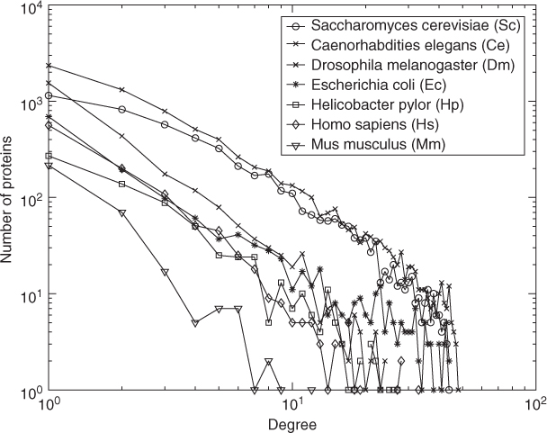
) follows a power law ![]() (and so is considered a scale-free network). This means that most vertices have low degrees,called low-shell proteins, and a few are highly connected, called hub proteins. Figure 18.1 shows the degree distributions of seven organisms in the DIP database [1]. The other feature is the small-world property, which is also known as 6 degrees of separation. This means that the diameter of the graph is small compared with the number of nodes.
(and so is considered a scale-free network). This means that most vertices have low degrees,called low-shell proteins, and a few are highly connected, called hub proteins. Figure 18.1 shows the degree distributions of seven organisms in the DIP database [1]. The other feature is the small-world property, which is also known as 6 degrees of separation. This means that the diameter of the graph is small compared with the number of nodes.
Figure 18.1 The degree distribution of 7 organisms in DIP database.
The standard tools to understand these networks are the clustering coefficient (Cc), the average pathlength, and the diameter of the network. The clustering coefficient (![]() ) is defined in terms of
) is defined in terms of ![]() , the set of edges in the neighborhood of
, the set of edges in the neighborhood of ![]() . The clustering coefficient is the probability that a pair of randomly chosen neighbors of
. The clustering coefficient is the probability that a pair of randomly chosen neighbors of ![]() are connected; that is
are connected; that is
18.24 ![]()
where ![]() is the neighborhood of
is the neighborhood of ![]() and
and ![]() are the edges in
are the edges in ![]() .
.
Since the denominator is the maximum possible number of edges between vertices connected to ![]() ,
, ![]() . The global clustering coefficient can be simply the average of all individual clustering coefficients (
. The global clustering coefficient can be simply the average of all individual clustering coefficients (![]() ) like
) like
18.25 
But this “average of an average” is not very informative [4]; one alternative is to weight each local clustering coefficient
18.26 
where MaxDeg is the maximum degree in the network. We use the latter Cc as our clustering coefficient for the rest of the chapter.
The pathlength of two nodes ![]() and
and ![]() is the smallest sum of edge weights of paths connecting
is the smallest sum of edge weights of paths connecting ![]() and
and ![]() . For an unweighted network, it is the smallest number of edges to go through. The average pathlength is the average of pathlengths of all pairs
. For an unweighted network, it is the smallest number of edges to go through. The average pathlength is the average of pathlengths of all pairs ![]() . The diameter of the network is the maximum pathlength.
. The diameter of the network is the maximum pathlength.
Because of the particular characteristics of PPI networks, a two-level approach has been proposed [32]. The main idea is derived from the ![]() -core concept introduced by Batagelj and Zaversnik [3]. If we repeatedly remove vertices of degree less than
-core concept introduced by Batagelj and Zaversnik [3]. If we repeatedly remove vertices of degree less than ![]() from a graph until there are no longer any such vertices, the result is the
from a graph until there are no longer any such vertices, the result is the ![]() -core of the original graph. The vertices removed are called the low-shell vertices. Then we remove the hub vertices; we choose a threshold
-core of the original graph. The vertices removed are called the low-shell vertices. Then we remove the hub vertices; we choose a threshold ![]() , and remove all vertices with degree
, and remove all vertices with degree ![]() . Pothen et al. [32] used
. Pothen et al. [32] used ![]() . The two-level approach factors in three assumptions in protein–protein interaction networks:
. The two-level approach factors in three assumptions in protein–protein interaction networks:
- The hub proteins interact with many other proteins, so it is difficult to limit them to only one cluster, and the computational complexity increases when they are included.
- There are many low-shell proteins, which increases the size of network. These nodes are easy to cluster when the nodes they are connected to are clustered first.
- Proteomic networks consist mostly of one large component and several small components.
Disregarding hub proteins and low-shell proteins, and limiting attention to the biggest component of proteomic networks leaves us to focus on the nodes that are most meaningful to cluster. Another advantage of this approach is that this architecture favors the size of the residual network, which requires less computational time.
18.5 Implementation of hierarchical methods
The hierarchical methods discussed here have three main phases:
The aggregation phase has traditionally been carried out using matching algorithms. This was the case with the early work of Oliveira and Seok on document clustering [26, 35]. Rather than use the more expensive maximal or maximum matching algorithms, cheaper greedy or random matching algorithms were used. Because of the high false positive rates in many PPI datasets, matchings can generate lower-quality coarsenings, which can yield lower-quality sets of clusters.
For PPI networks, because of their density and the lack of significant weighting, clique-based aggregation methods were developed. Cliques are sets of vertices in a graph where each pair of vertices in the set is connected by an edge of the graph. Cliques involve larger collections of edges, and so are less affected by high false positive rates. Below we describe some methods based on the use of triangular cliques, and also maximal cliques. As we look for larger cliques for performing the aggregation, both the complexity and the quality of the clusterings increases. How to balance the tradeoff between these aspects is a matter for future research.
After the clustering has been carried out for the coarsest graph in the hierarchy, the clusters must be disaggregated, possibly followed by application of a local method to refine the clustering. The use of a local method typically does not produce many changes, as they cannot “see” the effects of more radical changes to the clustering. However, local methods applied to quotient graphs can be much more effective: moving a vertex from one cluster to another in a quotient graph may represent the transfer of many nodes in the original graph between clusters. Applying refinement at each level of a hierarchy has the effect of “polishing” the cluster at all levels of coarsness. This can overcome problems of low quality in computationally cheap aggregation methods used to generate the hierarchy of graphs.
18.5.1 Matching-Based Methods
A matching in a graph is a set of edges of which no two are incident to the same node. Matchings provide a way of aggregating vertices into supernodes.
A matching is maximal when any edge in the graph that is not in the matching has at least one of its endpoints matched. Some algorithms aim to match as many nodes as possible, and some aim to maximize the sum of all edge weights [13, 39]; this is often referred to as maximum matching. These algorithms are too time-intensive and are designed for weighted graphs [23]. Instead, the algorithms below try to find a compromise between speed and quality.
The simplest matching for unweighted graphs is random matching. One node is randomly visited, and one of unmatched node is randomly chosen to be merged with the node [random vertex random merge (RVRM)]. A drawback is that the low-degree nodes have a higher chance of remaining unmatched than do high-degree nodes. Inorder to avoid this problem we can pick the lowest degree node among unmerged nodes and choose one of the unmerged nodes randomly to merge [lowest-degree vertex random merge (LVRM)]. Thus this algorithm tends to merge more nodes than RVRM.
We define the weights of edges as follows. The edge weights are initially all 1s to start but become the sum of the number of edges combined after one matching step. A node weight is defined as the total number of nodes merged into it.
When we have different edge weights we can apply the sorted matching (SM) concept for coarsening in subsequent levels. SM has been used for weighted graphs and merged nodes in order of decreasing edge weight [26]. In the PPI network, at first we have equal edge weights. We perform the first level of coarsening by combining nodes with each other, as long as they are not matched. The results are similar for any order that we select for this step. After this matching we will have groups of edges that share the same weight (the maximum resulting edge weight will be 4 for a clique with four nodes/vertices). We consider these groups in order of decreasing edge weight. Within each group we give higher priority to the edge with lower combined node weights; we take the edge with maximum ![]() as a tiebreak specifically, rule, where
as a tiebreak specifically, rule, where ![]() and
and ![]() are the node weights, that is, the number of nodes of supernodes
are the node weights, that is, the number of nodes of supernodes ![]() and
and ![]() . We call this matching scheme heavy edge small node (HESN).
. We call this matching scheme heavy edge small node (HESN).
Karypis et al. also present heuristic matching-based algorithms for unweighted networks [2]. Their heuristic algorithms were tested for power-law networks. Various algorithms are presented and experimentally compared. They reported that fewer within cluster edges are expected to be deleted when vertices are visited randomly, and one of the unmerged nodes is chosen in a greedy strategy. We include one of their coarsening algorithms in this research and compare it with ours. This random visit and merge greedy (RVMG) algorithm visits nodes randomly and a local greedy strategy is applied. In their greedy strategy, vertices that have connected edges with bigger edge weights are considered first. Smaller node weights are used to break ties for the same edge weights.
18.5.2 Clique-Based Methods
Triangular clique (TC)-based algorithms have been developed that merge highly connected triples of nodes [28]. A clique is a set of nodes in a graph where each node in the clique is connected to every other node in the clique by an edge of the graph. A triangular clique (TC) is a clique of three nodes (i.e., three nodes whose edges form a triangle). Our TC-based multilevel algorithm was inspired by Spirin and Mirny's use of cliques to identify highly connected clusters [37]. Our TC-based algorithm showed more proteins correctly merged into supernodes than any other matching based algorithm. This isbecause all three vertices in a TC have a very high chance of being part of the same functional module. A weakness of the TC-based algorithms is that there are many TCs in even a moderately sized clique. For example, there are 560 TCs in a clique of 16 nodes. Since we do not have efficient “matching” algorithms for TCs that avoid overlap, there are several choices as to how an algorithm treats a pair of TCs (see Ref. [25] and Fig. 18.2).
Figure 18.2 Four different TC-based coarsening algorithms. Each circle represents a node, and a triangle represents a supernode after coarsening.
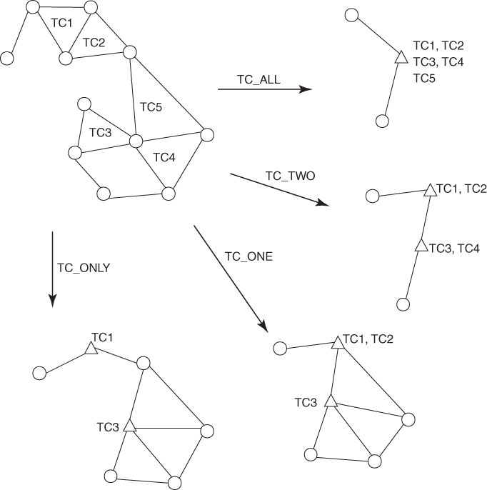
The various choices range from never combining connected TCs to form a single supernode (TC_ONLY) to always combining TCs that are connected (TC_ALL). In general, the more conservative approach (TC_ONLY and TC_ONE) gives more accurate clusters, but takes more time, than the more aggressive approaches (TC_TWO and TC_ALL).
Another more recent approach for identifying protein complexes used maximal cliques to create subgraphs with high densities [42]. Cliques are called maximal when they are not completely contained in another. In general, enumerating all maximal cliques takes much more time than finding all TCs. Fortunately, PPI networks are quite sparse, so all maximal cliques are enumerated quickly.
Our experimental results show that the quality of maximal cliques for finding protein complexes is very high. The bigger the maximal clique, the higher the quality of the results. This strongly motivates the use of maximal cliques in conjunction with multilevel algorithms. We can generalize TC-based multilevel algorithms to include maximal cliques. Note that the maximal cliques themselves do not identify clusters completely because cliques may have overlaps. Instead, they are used to quickly identify highly connected disjoint subgraphs. We call these approaches structure-based multilevel algorithms.
18.5.3 Refinement and Disaggregation
A traditional Kernighan–Lin (KL)-type refinement algorithm can be applied to improve the quality at each level [20], which has ![]() complexity. KL starts with an initial partition; it iteratively searches for nodes from each cluster of the graph if moving that node to one of the other clusters leads to a better partition. For each node, there may be more than one cluster giving a smaller objective function value than the current cut. So the node moves to the cluster that gives the biggest improvement. The iteration terminates when it does not find any node to improve the partition. However, this scheme has many redundant computations. For a given node
complexity. KL starts with an initial partition; it iteratively searches for nodes from each cluster of the graph if moving that node to one of the other clusters leads to a better partition. For each node, there may be more than one cluster giving a smaller objective function value than the current cut. So the node moves to the cluster that gives the biggest improvement. The iteration terminates when it does not find any node to improve the partition. However, this scheme has many redundant computations. For a given node ![]() , all clusters are considered as possible candidates to which the node
, all clusters are considered as possible candidates to which the node ![]() moves. Moving an edge to a cluster to which it is not already connected will always increase the number of edges between clusters. So we calculate the improvements for only those clusters that have edges with node
moves. Moving an edge to a cluster to which it is not already connected will always increase the number of edges between clusters. So we calculate the improvements for only those clusters that have edges with node ![]() . This modified scheme works much faster than traditional KL, especially for the sparse networks with large numbers of clusters. It should be mentioned that there are possibilities of certain objective functions that may improve when a node
. This modified scheme works much faster than traditional KL, especially for the sparse networks with large numbers of clusters. It should be mentioned that there are possibilities of certain objective functions that may improve when a node ![]() moves to a cluster that does have any edge with
moves to a cluster that does have any edge with ![]() . Note that it would be a good idea to find a faster refinement algorithm for multiway clustering such as the Fiduccia–Mattheyses linear time heuristic, which was used for bipartitioning problems [11].
. Note that it would be a good idea to find a faster refinement algorithm for multiway clustering such as the Fiduccia–Mattheyses linear time heuristic, which was used for bipartitioning problems [11].
The choice of the objective function may become important, as the structure of the objective function may make it possible to easily identify optimal vertices to swap, while other objective functions may make this task much harder. For example, if the objective function (to minimize) is the number of edges crossing between clusters, then the test for moving a vertex from cluster 1 to cluster 2 depends on whether the vertex has more edges to cluster 1 or to cluster 2. Efficient data structures can be created to track these numbers efficiently as the clusters are changed. However, if the objective function is more complex, such as ![]() from Equation (18.19), then determining suitable changes to the clustering may require substantially more computational effort.
from Equation (18.19), then determining suitable changes to the clustering may require substantially more computational effort.
18.6 Conclusion
Clustering problems, like other combinatorial optimization problems, are best tackled using a combination of discrete and continuous tools. Discrete methods (e.g., Kernighan–Lin methods and matching algorithms) are good for working with the local structure of a graph, while continuous methods (spectral clustering and SDP-based methods) are better at seeing the overall or global structure of the graph. The way to obtain optimal performance is likely to be combining them carefully to retain their strengths rather than their weaknesses. Continuous methods (such as spectral clustering) tend to be expensive on large graphs, while discrete methods (such as Kernighan–Lin) tend to be relatively cheap. Hierarchical methods where a graph is coarsened to create a sequence of quotient graphs, and where the coarsest of these is clustered using a continuous method, appear to offer the best compromise between computational cost and quality. Refinement of the clustering during the decoarsening phase of these algorithms seems to be especially useful in obtaining high-quality clusterings in reasonably computation time, even for very large graphs. Note that refinement should be guided by an objective function that is chosen to represent the task at hand, and not because it is convenient.
While there are different coarsening, decoarsening, and clustering algorithms, this framework of optimization-directed hierarchical methods has found success. Graphs with different structure may require different algorithms, but these algorithms have the potential to solve problems far beyond the ones for which they have already been used.
References
1. Database of Interacting Proteins (DIP) (available at http://dip.doe-mbi.ucla.edu/).
2. Abou-Rjeili A, Karypis G, Multilevel algorithms for partitioning power-law graphs, Proc. IEEE Int. Parallel & Distributed Processing Symp. (IPDPS), 2006.
3. Batagelj V, Zaversnik M, Generalized cores, in Computing Research Repository (CoRR), cs.DS/0202039, Feb. 2002 (available at http://arxiv.org/abs/cs.DS/0202039).
4. Bornholdt S, Schuster HG, eds., Handbook of Graphs and Networks, Wiley VCH, 2003.
5. Briggs WL, A Multigrid Tutorial. SIAM, Philadelphia, 1987.
6. Nguyen Bui TN, Jones C, Finding good approximate vertex and edge partitions is NP-hard, Inform. Process. Lett. 42(3):153–159 (1992).
7. Collette Y, Siarry P, Multiobjective optimization, in Decision Engineering, Springer-Verlag, Berlin, 2003 (principles and case studies).
8. De Bie T, Cristianini N, Fast SDP relaxations of graph cut clustering, transduction, and other combinatorial problems, J. Mach. Learn. Res. 7:1409–1436 (2006).
9. Ding C, He X, Zha H, Gu M, Simon H, A MinMaxCut Spectral Method for Data Clustering and Graph Partitioning, Technical Report 54111, Lawrence Berkeley National Laboratory (LBNL), Dec. 2003.
10. Dukanovic I, Rendl F, Semidefinite programming relaxations for graph coloring and maximal clique problems, Math. Program. B 109(2–3):S345–365 (2007).
11. Fiduccia CM, Mattheyses RM, A linear time heuristic for improving network partitions, Proc. 19th IEEE Design Automation Conf., Miami Beach, FL, pp. 175–181.
12. Fiedler M, Algebraic connectivity of graphs, Czech. Math. J. 23(98):298–305 (1973).
13. Gabow HN, Data structures for weighted matching and nearest common ancestors with linking, Proc. ACM-SIAM Symposium on Discrete Algorithms, 1990, pp. 434–443.
14. Garey MR, Johnson DS, Stockmeyer L, Some simplified NP-complete graph problems, Theor. Comput. Sci. 1:237–267 (1976).
15. Goemans MX, Semidefinite programming in combinatorial optimization, Math. Program. B79(1–3):143–161 (1997) [lectures on mathematical programming (ismp97) (Lausanne, 1997)].
16. Hagen L, Kahng A, Fast spectral methods for ratio cut partitioning and clustering, Proc. IEEE Int. Conf. Computer Aided Design, IEEE, 1991, pp. 10–13.
17. Jerrum M, Sorkin GB, Simulated annealing for graph bisection, Proc. 34th Annual Symp. Foundations of Computer Science, IEEE Comput. Soc. Press, Los Alamitos, CA, 1993, pp. 94–103.
18. Jerrum M, Sorkin GB, The Metropolis algorithm for graph bisection, Discrete Appl. Math. 82(1–3):155–175 (1998).
19. Karisch SE, Rendl F, Clausen J, Solving graph bisection problems with semidefinite programming, INFORMS J. Comput. 12(3):177–191 (2000).
20. Kernighan BW, Lin S, An efficient heuristic procedure for partitioning graphs, Bell Syst. Tech. J. 49(1):291–307 (1970).
21. Krogan N, et al, Global landscape of protein complexes in the yeast saccharomyces cerevisiae, Nature 440(7084):637–643 (2006).
22. McCormick SF, ed., Multigrid Methods, SIAM Frontiers in Applied Mathematics, Philadelphia, 1987.
23. Monien B, Preis R, Diekmann R, Quality matching and local improvement for multilevel graph-partitioning, Parallel Comput. 26(12):1609–1634 (2000).
24. Oliveira S, Seok SC, A matrix-based multilevel approach to identify functional protein models, Int. J. Bioinformatics Res. Appl. (in press).
25. Oliveira S, Seok SC, Multilevel approaches for large-scale proteomic networks, Int. J. Comput. Math. 84(5):683–695 (2007).
26. Oliveira S, Seok SC, A multi-level approach for document clustering, Lect. Notes Comput. Sci. 3514:204–211 (Jan. 2005).
27. Oliveira S, Seok SC, A multilevel approach for identifying functional modules in protein-protein interaction networks, Proc. 2nd Int. Workshop on Bioinformatics Research and Applications (IWBRA), Atlanta, GA, LNCS Series, Vol. 3992, 2006, pp. 726–773.
28. Oliveira S, Seok SC, Triangular clique based multilevel approaches to identify functional modules, Proc. 7th Int. Meeting on High Performance Computing for Computational Science (VECPAR), 2006.
29. Oliveira S, Stewart DE, Clustering for bioinformatics via matrix optimization, Proc. ACM-BCB'11 Conf. Bioinformatics, Computational Biology and Biomedicine, Chicago, Aug. 2011.
30. Peterson C, Anderson JR, Neural networks and NP-complete optimization problems; a performance study on the graph bisection problem, Complex Syst. 2(1):59–89 (1988).
31. Puig O, Caspary F, Rigaut G, Rutz B, Bouveret E, Bragado-Nilsson E, Wilm M, Séraphin B, The tandem affinity purification (TAP) method: A general procedure of protein complex purification, Methods 24(3):218–229 (2001).
32. Ramadan E, Osgood C, Pothen A. The architecture of a proteomic network in the yeast. Proc. CompLife2005, Lecture Notes in Bioinformatics, vol. 3695, pp. 265–276 2005.
33. Rao MR, Cluster analysis and mathematical programming, J. Am. Stat. Assoc. 66(335):622–626 (1971).
34. Reed BA, A gentle introduction to semi-definite programming, in Perfect Graphs, Wiley, Chichester, UK, 2001, pp. 233–259.
35. Seok SC, Multilevel Clustering Algorithms for Documents and Large-Scale Proteomic Networks, PhD thesis, University of Iowa, 2007.
36. Shi J, Malik J, Normalized cuts and image segmentation, IEEE Trans. Pattern Anal. Machine Intell. 22(8):888–905 (Aug. 2000).
37. Spirin V, Mirny LA, Protein complexes and functional modules in molecular networks, Proc. Natl. Acad. Sci. USA 100(21):12123–12128 (Oct. 2003).
38. Stewart GW, Building an Old-Fashioned Sparse Solver, Technical Report CS-TR-4527/UMIACS-TR-2003-95, Univ. Maryland, Sept. 2003.
39. Vazirani V, A theory of alternating paths and blossoms for proving correctness of the ![]() general graph maximum matching algorithm, Combinatorica 14(1):71–109 (1994).
general graph maximum matching algorithm, Combinatorica 14(1):71–109 (1994).
40. Wang J, Li M, Deng Y, Pan Y, Recent advances in clustering methods for protein interaction networks, BMC Genomics 11(S3):S10 (2010).
41. Yan JT, Hsiao PY, A fuzzy clustering algorithm for graph bisection, Inform. Process. Lett. 52(5):259–263 (1994).
42. Zhang C et al, Fast and accurate method for identifying high-quality protein-interaction modules by clique merging and its application to yeast, J. Proteome Res. 5(4):801–807 (2006).