
Chapter 7
Protein Structural Boundary Prediction
7.1 Introduction
At the present state of the art in protein bioinformatics, it is not yet possible to predict protein structure [43]. Proteins are among the major components of living organisms and are considered to be the working and structural molecules of cells. They are composed of building block units called amino acids [25, 34]. These amino acids dictate the structure of a protein [49].
Many machine learning approaches and new algorithms have been proposed to solve the protein structure prediction problem [5, 7, 13, 15, 31, 41]. Among the machine learning approaches, support vector machines (SVMs) have attracted a lot of attention because of their high prediction accuracy [1]. Since protein data consist of sequence and structural information, another widely used approach for modeling these structured data is to analyze them as graphs. In computer science, graph theory has been widely studied; however, more recently it has been applied to bioinformatics. In out research, we introduced new algorithms based on statistical methods, graph theory concepts, and machine learning for the protein structure prediction problem.
In this chapter, we describe a novel encoding scheme and a computational method using machine learning for prediction starting and ending points of secondary structure elements. Most computational methods have been developed with the goal to predict the secondary structure of every residue in a given protein sequence. However, instead of predicting the structure of each and every residue, a method that can correctly predict where each secondary structure segment (e.g., α helices, β sheets, or coils) in a protein starts and ends could be much more reliable since fewer predictions would be required. Our system makes only one prediction to determine whether a given sequence segment is the start or end of any secondary structure H, E, or C, whereas the traditional methods must be able to predict each and every residue's structure correctly in the segment in order to make that decision. We compared the traditional existing binary classifiers to the new binary classifiers proposed in this chapter and achieved an accuracy much higher than that of the traditional approach.
In summary, we propose methods for predicting protein secondary structure and detecting transition boundaries of secondary structures of helices (H), coils (C), and sheets (E). Detecting transition boundaries instead of the structure of individual residues in the whole sequence is much easier. Thus, our problem is reduced to the problem of finding these transition boundaries.
7.2 Background
In this chapter, we present problem definitions and discuss our motivation for research, and related work. This section gives a general background for the methods that we propose.
7.2.1 Prediction of Protein Structure
Proteins are polymers of amino acids containing a constant mainchain (linear polymer of amino acids) or backbone of repeating units with a variable sidechain (sets of atoms attached to each α carbon of the mainchain) attached to each [33]. Proteins play a variety of roles that define particular functions of a cell [33]. They are a critical component of all cells and are involved in almost every function performed by them. Proteins are building blocks of the body controls; they facilitate communication with cells and transport substances. Biochemical reactions among enzymes also contain protein. The transcription factors that turn genes on and off are proteins as well.
A protein consists primarily of amino acids, which determine its structure. There are 20 amino acids that can produce countless combinations of proteins [25, 36]. There are four levels of structure in a protein:
Figure 7.1 CASPASE 7 protein.
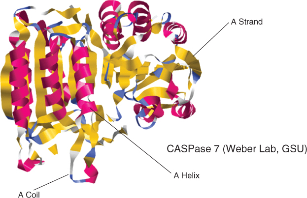
Many proteins contain more than one polypeptide chain; the combinations two or more polypeptide chains in a protein make up its quaternary structure [9, 18]. The protein in Figure 7.1 is a CASPase 7 protein borrowed from the Weber lab in the Georgia State University (GSU) Biology Department.
Proteins interact with DNA (deoxyribonucleic acid), RNA (ribonucleic acid), and other proteins in their tertiary and quaternary states. Therefore, knowing the structure of a protein is crucial for understanding its function.
Large volumes of genes have been sequenced more recently. Therefore, the gap between known protein sequences and protein structures that have been experimentally determined is growing exponentially. The Protein Data Bank (PDB) [10] contains many proteins whose amino acid sequences are known; however, only a small fraction of these protein structures are known [7, 10] because nuclear magnetic resonance (NMR) and X-ray crystallographic techniques take years to determine the structure of one protein. Therefore, access to computational tools to predict the structure of a protein is very important and necessary. Although only a few of the computational methods proposed for protein structure prediction yield 100% accurate results, even an approximate model can help experimental biologists guide their experiments. The ability to predict the secondary and tertiary structures of a protein from its amino acid sequence is still a major challenge in bioinformatics. With the methods available today, protein tertiary structure prediction is a very difficult task even when starting from exact knowledge of protein backbone torsion angles [11]. It has also been suggested that protein secondary structure delimits the overall topology of the proteins [35]. It is believed that predicting the protein secondary structure provides insight into, and an important starting point for, prediction of the tertiary structure of the protein, which leads to understanding the function of the protein. There have been many approaches toward revealing the protein secondary structure from the primary sequence information [17, 22, 37–40, 50, 51].
7.2.2 Protein Secondary Structure Prediction Problem Formulation
In this work, we adopted the most generally used Dictionary of Secondary Structure of Proteins (DSSP) secondary structure assignment scheme [29]. The DSSP classifies the secondary structure into eight different classes: H (α helix), G (310 helix), I (π helix), E (β strand), B (isolated β bridge), T (turn), S (bend), and—(rest). These eight classes were reduced for the purposes of this work into three regular classes based on the following method: H, G, and I, to H; E, to E; and all others, to C. In this work, H represents helices; E represents sheets and C represents coils.
The formulation in stated is Problem 7.1.
The quality of secondary structure prediction is measured with a three-state accuracy score denoted as Q3. The Q3 formula is the percent of residues that match reality as follows:
7.1 
The Q3 index is one of the most commonly used performance measures in protein secondary structure prediction. It refers to the three-state overall percentage of correctly predicted residues.
7.2.3 Previous Work on Protein Secondary Structure Prediction
The protein secondary structure prediction problem has been studied widely for almost 25 years. Many methods have been developed for the prediction of secondary structure of proteins. In the initial approaches, secondary structure predictions were performed on single sequences rather than families of homologous sequences [21]. The methods were shown to be ∼65% accurate. Later, with the availability of large families of homologous sequences, it was found that when these methods were applied to a family of proteins rather than a single sequence, the accuracy increased well above 70%. Today, many proposed methods utilize evolutionary information such as multiple alignments and PSI-BLAST profiles [2]. Many of those methods that are based on neural networks, SVM, and hidden Markov models have been very successful [5, 7, 13, 15, 31, 41]. The accuracy of these methods reaches ∼80%. An excellent review of the methods for protein secondary structure prediction has been published by Rost et al. [41].
7.2.4 Support Vector Machines
The support vector machines (SVM) algorithm is a modern learning system designed by Vapnik and Cortes [46]. Based on statistical learning theory, which explains the learning process from a statistical perspective, the SVM algorithm creates a hyperplane that separates the data into two classes with the maximum margin. Originally, it was a linear classifier based on the optimal hyperplane algorithm. However, by applying the kernel method to the maximum-margin hyperplane, Vapnik and his colleagues proposed a method for building a nonlinear classifier. In 1995, Cortes and Vapnik suggested a soft-margin classifier, which is a modified maximum-margin classifier that allows for misclassified data. If there is no hyperplane that can separate the data into two classes, the soft-margin classifier selects a hyperplane that separates the data as cleanly as possible with a maximum margin [16].
Support vector machine learning is related to recognizing patterns from the training data [1, 19]. The SVM software program SVMlight is an implementation of SVMs in C [26]. In this chapter, we adopt this SVMlight software, which is an implementation of Vapnik's SVMs [45]. This software also provides methods for assessing the generalization performance efficiently.
SVMlight consists of a learning module (svm_learn) and a classification module (svm_classify). The classification module can be used to apply the learned model to new examples.
The format for training data and test data input file is as follows:
 <line> .=. <target> <feature>:<value> <feature>:<value> …
 <target> .=. +1 | −1 | 0 | <float>
 <feature> .=. <integer> | “qid”
 <value> .=. <float>
For classification, the target value denotes the class of the example; +1 and −1, as the target values, denote positive and negative examples, respectively.
7.3 New Binary Classifiers for Protein Structural Boundary Prediction
Proteins consist primarily of amino acids, which determine the structure of a protein. Protein structure has three states: primary structure, secondary structure, and tertiary structure. The primary structure of the protein is its amino acid sequence; the secondary structure is formed from recurring shapes: α helix, β sheet, and coil. The tertiary structure of the protein is the spatial assembly of helices and sheets and the pattern of interactions between them. Predicting the secondary and tertiary structures of proteins from their amino acid sequences is an important problem; knowing the structure of a protein aids in understanding how the functions of proteins in metabolic pathways map for whole genomes, in deducing evolutionary relationships, and in facilitating drug design.
It is strongly believed that protein secondary structure delimits the overall topology of the proteins [21] Therefore, since the mid-1980s, many researchers have tried to understand how to predict the secondary structure of a protein from its amino acid sequence. Many algorithms and machine learning methods have been proposed for this problem [2, 30, 32]. The algorithms for predicting secondary structure of proteins have reached a plateau of roughly 90%. Much more success has occurred with motifs and profiles [15].
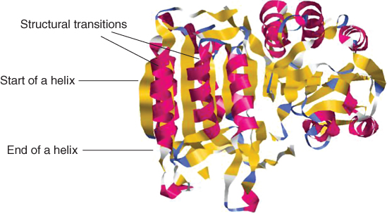
The common approach to solve the secondary structure prediction problem has been to develop tools that predict the secondary structure for each and every amino acid (residue) of a given protein sequence. Here, we propose new binary classifiers that do not require the correct prediction of each and every residue in a given protein segment. The new binary classifiers predict only the start or end of a helix, sheet or coil. We illustrated this concept in Figure 7.2, which is a schematic representation of the tertiary structure of a protein with its secondary structure regions colored in different shades. The point where one secondary structure element ends and another one begins is called a structural transition throughout this chapter.
Figure 7.2 Structural transitions of a protein.
Protein sequences may have specific residue preferences at the end or start of secondary structure segments. For example, it has been shown that specific residue preferences exist at the end of helices, which is called helix capping. More recent research has suggested that it is possible to detect helix capping motifs [6]. However, these results reflect a linear decision function based on amino acid frequencies. It is well known that nonlinear decision functions, for example, those implemented with support vector machines (SVMs), dramatically outperform linear decision functions when the underlying data are nonlinear [46]. In this work, we use a machine learning approach based on SVM to predict the helix capping regions of a given protein sequence. These helix capping regions indicate where a helix ends. The same method is also used for predicting the start points of helices and to predict the endpoints and startpoints of coils and sheets. The ending and starting points of secondary structures are also called structural transition boundaries.
7.3.1 Problem Formulation
In this study, we adopted the most generally used DSSP secondary structure assignment scheme [29]. As mentioned in Section 7.2.2, the eight classes were reduced into three regular classes based on the following method: H, G, and I were reduced to H; E, to E; and all others, to C.
7.3.1.1 Traditional Problem Formulation for Secondary Structure Prediction
The traditional problem formulation is stated as exactly the same as Problem 7.1.
Given a protein sequence a1a2…aN, find the state of each amino acid ai as being either H (helix), E (strand), or C (coil).
As mentioned earlier, the metric Q3 is used to measure the quality of the secondary structure prediction. The Q3 score, which is termed three-state accuracy, represents the percent of residues that match reality. Most of the previous research adopted Q3 as an accuracy measurement.
7.3.1.2 New Problem Formulation for Transition Boundary Prediction
The new problem formulation is stated as follows.
Here, we used a new scoring scheme that we call QT (where T denotes transition), which is similar to Q3; however, QT is the percent of residues that match reality. We had to change the scoring scheme to QT because the Q3 scoring scheme takes into account all the residues whereas QT factors in only the residues that are necessary for prediction.
7.2 
In the QT scoring scheme, the number of correctly predicted transition residues of class H, E, or C is divided by the number of all transition residues of class H, E, or C.
7.3.2 Method
7.3.2.1 Motivation
Given a protein sequence of a 9-mer, let the middle element of this 9-mer be the starting position of a helix as shown in Figure 7.3. Our goal is to determine whether the middle residue is the start or end of a helix. If we use the traditional binary classifiers (such as H/∼H), first we must correctly identify all the residues in the whole segment. We need to correctly predict three consecutive residues as H (at least four residues are needed for a helix), and the remaining residues should be ∼H. In this case, we have to make nine predictions, and ideally we should be correct all 9 times. However, the probability that we can predict all nine residues correctly in the protein segment is at maximum 0.35 if we assume that our chance of making each prediction correctly is 0.9 and that this probability of success is independent of the other predictions.
Figure 7.3 A 9-mer with helix junction.
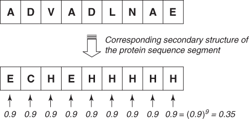
In the next section, we explore how to overcome the problem of making nine predictions for a given 9-mer and how to reduce it to a problem of making only one prediction per 9-mer.
7.3.2.2 A New Encoding Scheme for Prediction of Starts of H, E, and C
The goal of our new encoding scheme is shown in Figure 7.4, where a new binary classifier has to make only one guess instead of nine guesses. Here, the new encoding scheme for representing the starting points of helices is shown as an example. The same encoding is applied to both sheets and coils.
Figure 7.4 New encoding scheme for the helix startpoint.
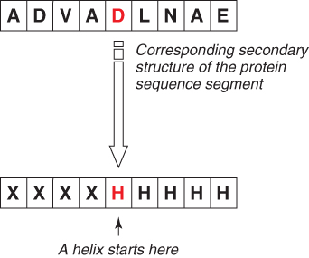
Figure 7.4 illustrates the new encoding scheme.
For the middle residue to be classified as the start of a helix, the rules of the new encoding scheme are as follows:
If all three rules are satisfied, the protein segment is represented by the new encoding scheme as the start of a helix (Hstart). If not, the protein segment is represented as ∼Hstart (not the start of a helix).
7.3.2.3 A New Encoding Scheme for Prediction of Ends of H, E, and C
Similar to the the method described in Section 7.3.2.2, the new encoding scheme for representing the ends of helices is shown as an example is in Figure 7.5. The same encoding is applied to sheets and coils.
Figure 7.5 A 9-mer with helix end.

In the new encoding scheme, the protein sequences are classified as shown in Figure 7.6.
Figure 7.6 New encoding scheme for helix start.
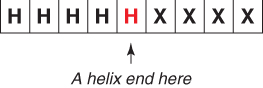
The rules of the new encoding scheme are listed below. These are similar to the rules listed in Section 7.3.2.2, but are used to predict the ends of secondary structures. For the middle residue to be classified as a helix end, the conditions are as follows:
If all three rules are satisfied, the protein segment is represented by the new encoding as the end of a helix (![]() ). If not, the protein segment is represented as ∼Hend (not the end of an helix).
). If not, the protein segment is represented as ∼Hend (not the end of an helix).
7.3.3 New Binary Classifiers
In the traditional secondary structure prediction approach, usually six binary classifiers, such as three “1 versus rest” classifiers (H/∼H, E/∼E, and C/∼C) and three “1 versus 1” classifiers (H/E, E/C, and C/H) are used. Here, the numeral 1 in the “1 versus rest” classifier refers to a positive class and the term rest indicates a negative class. Likewise, the expression “1's in 1 versus 1” classifier refers to positive class and negative class, respectively. For example, the classifier H/∼H classifies the testing sample as helix or not helix, and the classifier E/C classifies the testing sample as sheet or coil.
The following six new binary classifiers are proposed:
7.3.4 SVM Kernel
We used a radial basis function (RBF) kernel because it was optimal when used for secondary structure prediction:
7.3 ![]()
Here, x and y are two input vectors containing different feature values and γ is the radial basis kernel parameter. Radial basis kernels depend on a numerical representation of the input data.
7.3.5 Selection of Window Size
In order to choose an optimal window size for the proposed encoding scheme for a given protein segment, we tried different window sizes on the smaller dataset RS126. We used the position-specific scoring matrix (PSSM) profiles of the dataset RS126 during the tests. As a prediction method, we used the SVM RBF kernel. Using the sliding-window scheme, we extract first each k-mer from a protein sequence. Each k-mer is classified as a positive or negative sample. If the middle residue satisfies the encoding scheme as described in Section 7.3.2, it is marked as a positive sample: Hstart, Estart, or Cstart. Otherwise it is marked as a negative sample: ∼Hstart, ∼Estart, or ∼Cstart,
Figure 7.7 shows the QT prediction accuracy results of all the six new binary classifiers used with the SVM RBF kernel and the RS126 dataset. The prediction accuracy of SVM varied for different window sizes. The best overall prediction accuracy was achieved with window size 9.
Figure 7.7 Accuracy of Hend, Eend, and Cend binary classifiers for the RS126 dataset.
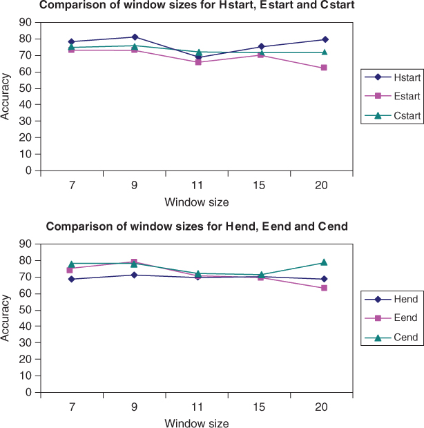
Figure 7.8 shows the QT prediction accuracy results of all the six new binary classifiers used with the SVM RBF kernel and the CB513 dataset. The prediction accuracy of SVM varied for different window sizes. The best overall prediction accuracy was achieved when the window size was 9 for CB513 data, which is similar to the results of RS126 data shown in Figure 7.7.
Figure 7.8 Accuracy of Hend, Eend, and Cend binary classifiers for CB513 dataset.
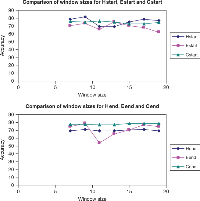
For the latter experiments and for the larger CB513 dataset, a window size of 9 was used to test the new binary classifiers.
7.3.6 Test Results of Binary Classifiers
Table 7.1 shows the QT prediction accuracy results of all six binary classifiers Hstart/∼Hstart, Estart/∼Estart, Cstart/∼Cstart and Hend/∼Hend, Eend/∼Eend and Cend/∼Cend used with the SVM RBF kernel with a window size of 9. We used the PSSM profiles of the dataset CB513 during these tests. Since there were many negative samples, we balanced the negative and positive samples in the dataset by randomly choosing from the negative samples for training the SVM. The results are given in Table 7.1. The probability of SVM correctly predicting the start of helices is 81.5%, which is much higher than the 35% theoretical bound for per-residue prediction. The probability of successfully predicting the end of a helix is also high—approximately 71.33%. This shows that there is more of a signal in the data indicating the start of helices than there is a stop signal. The start and end positions of strands and coils are predicted with approximately 75% accuracy.
Table 7.1 Prediction Accuracies of the New Binary Classifiers
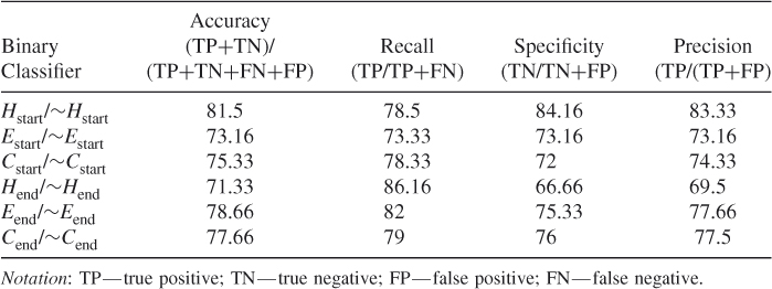
These results show that, by training a classifier such as SVM to predict the secondary structure transition boundaries, one can detect where helices, strands, and coils begin and end with high accuracy. Furthermore, these secondary structure transition boundaries are detected in an attempt to perform only one prediction at a time rather than trying to predict correctly all the residues in a given sequence segment, the probability of which would theoretically be only roughly 35%.
7.3.7 Accuracy as a Function of Helix Size
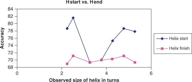
Figure 7.9 compares the prediction accuracy levels of helix starting and ending points as a function of the number of turns in the helix. One can see that the prediction accuracies of the binary classifiers Hstart/∼Hstart and Hend/∼Hend reach a maximum value when the helix has 2.25 turns. Since a helix has about 4 residues per turn, this corresponds to a window size of 9 residues. At different number of turns of a helix, the accuracies are lower. This also proves that choosing a window size of 9 residues is optimal for the transition boundary prediction problem.
Figure 7.9 Accuracy levels of Hstart and Hend.
7.3.8 Comparison between Traditional Binary Classifiers and New Binary Classifiers
Several studies focus on determining where the structural segments start and end. Aydin et al. have shown that new dependence models and training methods bring further improvements to single-sequence protein secondary structure prediction [7]. Their results improve most Q3 accuracy results by 2%, which shows that considering amino acid patterns at segment borders increases the prediction accuracy. Some other approaches focus on finding the end of helices. The reason for this is that the helices (α-helices) are the most abundant regular secondary structure and that a certain residue preference exists at the ends of helices [48]. However, current secondary structure prediction programs cannot identify the ends of helices correctly in most cases. The same rule applies to strands, although the residue preferences for strand termini are not as strong as in helices. Wilson et al. used cumulative pseudo-free-energy calculations to predict helix start positions and achieved 38% prediction accuracy. We achieved ∼80% QT accuracy using SVM, which is, of course, significantly higher.
One could question what our Q3 overall prediction accuracy is. Most of the current secondary structure prediction methods attempt to solve the problem at a perresidue level, whereas we try to solve the prediction at a persegment level. In this work, we proposed binary classifiers that target prediction of the start and end positions of helices, strands, and coils. Therefore, to compare our prediction accuracy to the current prediction methods, we derived a method that converts our QT accuracy results to the standard Q3 and vice versa.
7.3.8.4 Estimates of Q3 from QT and QT from Q3
When traditional binary classifiers such as “1 versus rest” classifiers (H/∼H, E/∼E, and C/∼C), and “1 versus 1” classifiers (H/E, E/C, and C/H) are used, their prediction accuracies are measured using a Q3 metric. In the Q3 measurement, predictions for each and every residue of a protein sequence are performed. To determine whether a given protein sequence is the start or end of a secondary structure with the traditional binary classifiers, each residue's secondary structure must be predicted first. However, it is clear that, even with the 90% accuracy per residue, the probability of independently predicting k residues correctly is 0.9 to the kth order. In order to calculate a Q3 measurement of a given protein sequence window (of size k), a prediction for each and every residue in that window must be made using the traditional binary classifiers. However, with the proposed new binary classifiers, only one prediction per window is suffices to indicate whether that window represents the end or start of a helix, sheet, or coil. Besides, the overall prediction probability is slightly pessimistic because the estimates may not be fully independent.
In light of this reasoning, to compare our results to those of the traditional binary classifiers that calculate the prediction accuracy per residue, we derived a method using the following assumption. Given a protein segment of window size k, we assumed that the prediction of each residue in that window is truly independent of the other residues in that window. Then, we converted the traditional Q3 accuracy measurement to our accuracy measurement QT, using the following equation:
7.4 ![]()
This formula basically states that the fewer the number of predictions made for a given protein window, the higher the chances are that the prediction is correct. Using the traditional binary classifiers, given a protein window of size k, we must make k predictions to see what that protein sequence segment is. Using the binary classifiers proposed in this work, only one prediction is enough. The inverse of Equation (7.3) is
5 ![]()
The inverse of this formula gives us the corresponding Q3 accuracy as a function of QT.
7.3.8.5 Traditional Versus New Binary Classifiers
In order to make a fair comparison, we took Q3 measurements for the H/∼H, E/∼E, and C/∼C binary classifiers from References 23 and 24, which provide one of the highest Q3 measurements for these binary classifiers, and estimated their QT measurements. We also converted the QT results in Table 7.1 to Q3 measurements and listed the results in Tables 7.2 and 7.3.
Table 7.2 Estimated Q3 Results
| QT Converted to Q3 | ||
| Binary Classifiers | QT | Q3 |
| H/∼H | 83.17 | 96.31 |
| E/∼E | 80.5 | 95.67 |
| C/∼C | 76.5 | 94.65 |
Table 7.3 Estimated QT Results
| Q3 Converted to QT | ||
| Binary Classifiers | Q3 | QT |
| H/∼H | 87.18 | 50.35 |
| E/∼E | 86.02 | 47.09 |
| C/∼C | 77.47 | 36.01 |
Sources: Q3 measurements from Hu et al. [23] and Hua and Sun [24].
Table 7.2 shows our QT accuracy calculations converted to the corresponding Q3 accuracies. When Q3 accuracies are converted to QT measurements as shown in Table 7.3, the accuracies are low. (Note: These estimates are based on the assumption that each residue prediction is independent of all the others.) These results show that using the new binary classifiers gives prediction accuracy higher than that obtained using the traditional binary classifiers. These results also prove that it is better to make predictions using a per segment window rather than per residue. In other words, we should split the data into large chunks (segments) and make predictions using these segments instead of attempting to predict each and every piece of data (residues).
7.3.9 Test Results on Individual Proteins Outside the Dataset
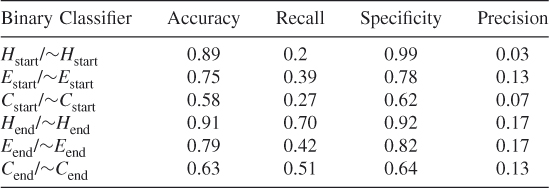
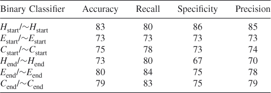
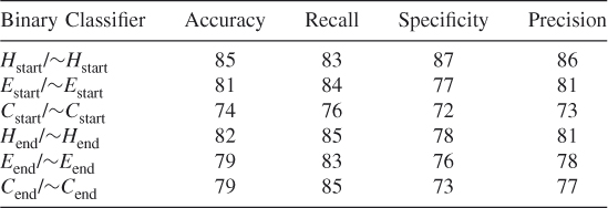
In order to prove that the new proposed encoding scheme works, we have run double-blind tests on individual proteins. The test results are given in Table 7.4. In all test cases, the accuracy, recall and specificity values are high as expected; however, the precision values are low (see also Tables 7.8–7.6). This is due to the unbalanced nature of the dataset. In our training datasets, we have many negative samples whereas the positive samples constitute roughly 1% of the number of the negative sets. This is a major problem with these kinds of datasets. The false positives (FPs) are high because we are dealing with 100 times more examples of negative cases than positive cases. These results imply that it is very difficult to obtain a high precision, because of the unbalanced nature of the datasets. The false positives overwhelm the correct matches. This is the truly difficult aspect of using minority classes. The good accuracy shows that there is a signal in the data that we can extract. However, because there are so many more negative matches, we obtain a large number of FPs. What we discover by this analysis is that there is a signal that SVM selects because we have high accuracy; however, we cannot obtain high precision values because there are very few examples of the minority classes. Therefore, we give the results for both balanced data and unbalanced data.
Table 7.4 Protein ID: CBG
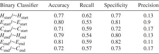
Table 7.5 Protein ID: BAM
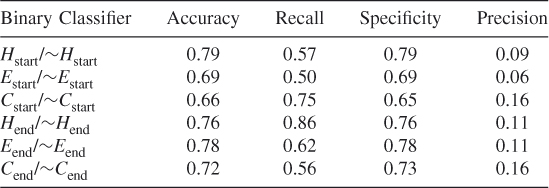
Table 7.6 Protein ID: ADD1
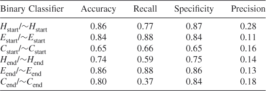
Table 7.7 Protein ID: AMP1
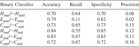
Table 7.8 Protein ID: CELB
7.3.10 Test Results on Randomly Selected Data Subsets
In order to ensure that we did not simply select a subset of the negative data for balancing the dataset that optimized our method's prediction probabilities, we tested our method using 10 different randomly chosen different subsets of the data. These test results show that our proposed method works and that it is possible to train an SVM algorithm to learn where the helices, strands, and coils begin and end. (See Tables 7.9–7.18.)
Table 7.9 Test 1, Random Subset 1
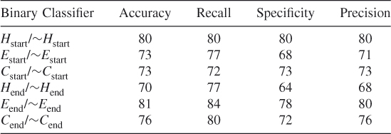
Table 7.10 Test 2, Random Subset 2
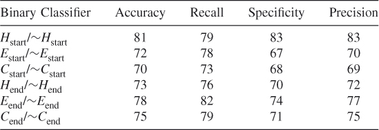
Table 7.11 Test 3, Random Subset 3
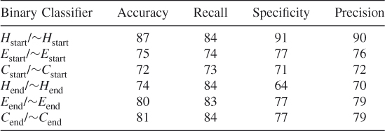
Table 7.12 Test 4, Random Subset 4
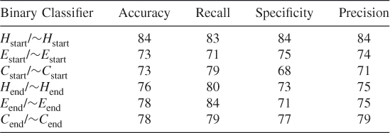
Table 7.13 Test 5, Random Subset 5
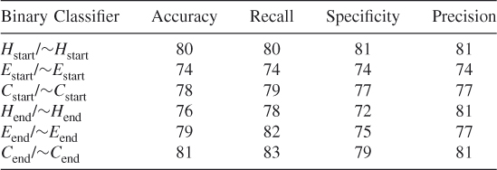
Table 7.14 Test 6, Random Subset 6
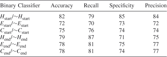
Table 7.15 Test 7, Random Subset 7
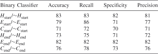
Table 7.16 Test 8, Random Subset 8
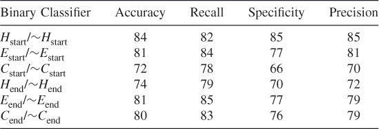
Table 7.17 Test 9, Random Subset 9
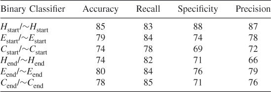
Table 7.18 Test 10, Random Subset 10
7.3.11 Additional Test Results on Randomly Selected Data Subsets
To ensure that we did not simply select a subset of the data that optimized our method's prediction probabilities when we balanced the dataset, we tested our method using 10 different randomly chosen different subsets of the data. These test results show that our proposed method works and that it is possible to train an SVM algorithm to learn where the helices, strands, and coils begin and end when features are reduced according to the clique algorithm. (See Tables 7.19–7.28.)
Table 7.19 Test 1, Random Subset 1
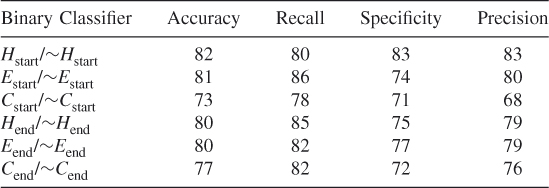
Table 7.20 Test 2, Random Subset 2
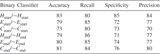
Table 7.21 Test 3, Random Subset 3
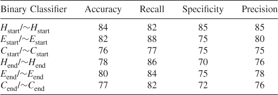
Table 7.22 Test 4, Random Subset 4
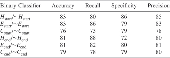
Table 7.23 Test 5, Random Subset 5
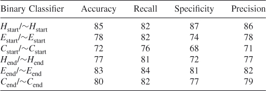
Table 7.24 Test 6, Random Subset 6
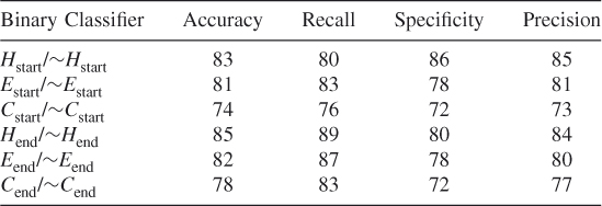
Table 7.25 Test 7, Random Subset 7
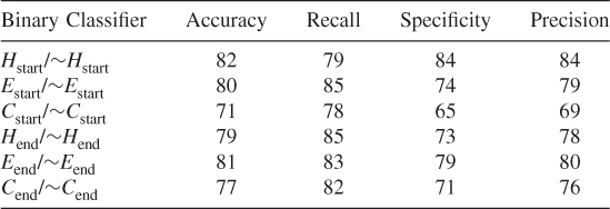
Table 7.26 Test 8, Random Subset 8
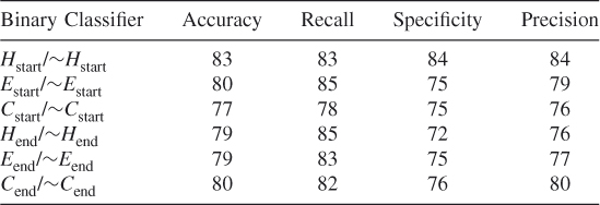
Table 7.27 Test 9, Random Subset 9
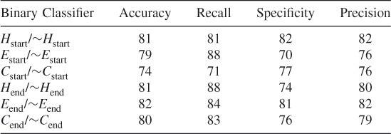
Table 7.28 Test 10, Random Subset 10
7.3.12 Conclusion
In this section, we proposed a new way to look at the protein secondary prediction problem. Most of the current methods use the traditional binary classifiers such as H/∼H and require the correct prediction of every residue's secondary structure. This approach gives an overview of the secondary structure of a sequence. However, to determine whether a sequence segment is a helix, sheet, or coil using the traditional binary classifier, most of the residues in the sequence segment must be classified correctly. Even with a 90% probability that each residue is correctly predicted independently, the cumulative probability of being correct for all the residues in the sequence segment is low (∼35%). We propose six new binary classifiers that could be used to classify all the residues in a given protein sequence segment when attempting to determine whether the sequence segment is a helix, strand, or coil. In our binary classifiers, only one classification is made per segment. To apply these binary classifiers, we proposed a new encoding scheme for data representation. Our results show that it is possible to train an SVM to learn where the helices, strands, and coils begin and end.
We proposed six new binary classifiers that are used to predict the starts and end of secondary structures of protein. For these binary classifiers, we also proposed a new encoding scheme. Our current encoding scheme takes into account only the information as to whether a protein window is the end or start of a secondary structure. It does not factor in where in the protein that sequence window belongs. Depending on whether it occurs at the beginning or end of a sequence, the occurrence of a transition boundary could be changed drastically. The new binary classifiers currently do not use the information that stipulates that a sequence window be at the start or end of protein; however, these classifiers can be improved in the future to represent this information.
Another future improvement could be to find common amino acid patterns that make up the transition boundaries. If there are common amino acid patterns (motifs), this information could be added to the encoding scheme and an SVM could be additionally trained with these patterns to ensure a more accurate prediction. These common patterns could lead to rules stipulating, for instance, order in which amino acids represent transition boundaries. These rules can later be embedded into the encoding scheme or put into a new kernel function of SVM.
The correct detection of transition boundaries could be used to predict the tertiary structure of a protein. For instance, each transition boundary could also be a possible domain boundary. Proteins usually contain several domains or independent functional units that have their own shape and function. All these remain as promising topics for future research.
7.4 Conclusion
We propose six new binary classifiers that are used for predicting the start and end of secondary structures of protein. With these binary classifiers, it is easier to train an SVM since only one prediction per protein segment is necessary for concluding whether it is a helix, strand, or coil. In order to use these binary classifiers, we also proposed a new encoding scheme for data representation. Our results show that it is possible to train an SVM to learn where the helices, strands, and coils begin and end. We have achieved close to 90% accuracy, whereas traditional binary classifiers can attain a maximum only accuracy of only 35% for a window size of 9.
Detecting transition boundaries instead of the structure of individual residues in the whole sequence is much easier. Thus, our problem is reduced to the task of finding these transition boundaries. Our work provides new insights on accurately prediction of protein secondary structure and may help determine tertiary structure as well; this could be used by biologists to help solve the critically important problem of how proteins fold. A protein's tertiary structure is critical to its ability to perform its biological functions correctly and efficiently.
References
1. Abe S, Support Vector Machines for Pattern Classification, Springer-Verlag, 2005.
2. Altschul SF, Madden TL, Schaffer AA, Zhang J, Zhang Z, Miller W, Lipman DJ, Gapped BLAST and PSI-BLAST: A new generation of protein database search programs, Nucleic Acids Res. 25(17):3389–3402 (1997).
3. Altschul SF, Gish W, Miller W, Myers EW, Lipman DJ, Basic local alignment search tool, J. Mol. Biol. 215(3):403–410 (1990).
4. Altun G, Zhong W, Pan Y, Tai PC, Harrison RW, A new seed selection algorithm that maximizes local structural similarity in proteins, Proc. Int. IEEE Conf. Engineering in Medicine and Biology (EMBC'06), Aug. 2006, pp. 5822–5825.
5. Altun G, Hu H-J, Brinza D, Harrison RW, Zelikovsky A, Pan Y, Hybrid SVM kernels for protein secondary structure prediction, Proc. Int. IEEE Conf. Granular Computing (GRC 2006), May 2006, pp. 762–765.
6. Aurora R, Rose G, Helix capping, Protein Sci. 7:21–38 (1998).
7. Aydin Z, Altunbasak Y, Borodovsky M, Protein secondary structure prediction for a single-sequence using hidden semi-Markov model, BMC Bioinformatics. 7(1):178 (2006).
8. Baxevanis AD, Ouellette BF. Bioinformatics: A Practical Guide to the Analysis of Genes and Proteins, Wiley, 2005.
9. Berg JM, Tymoczko JL, Stryer L, Biochemistry, 5th ed., Freeman WH, New York, 2002.
10. Berman H, Henrick K, Nakamura H, Markley JL, The worldwide Protein Data Bank (wwPDB): Ensuring a single, uniform archive of PDB data, Nucleic Acids Res. 35: (Jan. 2007).
11. Birzele F, Kramer S, A new representation for protein secondary structure prediction based on frequent patterns, Bioinformatics, 22(21):2628–2634 (2006).
12. Butenko S, Wilhelm W, Clique-detection models in computational biochemistry and genomics, Eur. J. Oper. Res. 17(1):1–17 (2006).
13. Breiman L, Random forests, Machine Learn. 45(1):5–32 (2001).
14. Breiman L, Cutler A, Random forest (available at http://www.stat.berkeley.edu/∼breiman/RandomForests/cc_software.htm).
15. Bystroff C, Thorsson V, Baker D, HMMSTR: A hidden Markov model for local sequence structure correlations in proteins, J. Mol. Biol. 301:173–190 (2000).
16. Burges C, A tutorial on support vector machines for pattern recognition, Data Mining Knowl. Discov. 2(2):121–167 (1998).
17. Casbon J, Protein Secondary Structure Prediction with Support Vector Machines, MSc thesis, Univ. Sussex, Brighton, UK, 2002.
18. Chou PY, Fasman GD, Prediction of protein conformation, Biochemistry 13(2):222–245 (1974).
19. Cristianini N, Shawe-Taylor J, An Introduction to Support Vector Machines, Cambridge Univ. Press, 2000.
20. Efron B, Tibshirani R, An Introduction to the Bootstrap, Chapman & Hall, New York, 1993.
21. Fleming PJ, Gong H, Rose GD, Secondary structure determines protein topology, Protein Sci. 15:1829–1834, (2006).
22. Garnier J, Osguthorpe DJ, Robson B, Analysis of the accuracy and implications of simple methods for predicting the secondary structure of globular proteins, J. Mol. Biol. 120:97–120 (1978).
23. Hu H, Pan Y, Harrison R, Tai PC, Improved protein secondary structure prediction using support vector machine with a new encoding scheme and an advanced tertiary classifier, IEEE Trans. Nanobiosci. 3(4):265–271 (2004).
24. Hua S, Sun Z, A novel method of protein secondary structure prediction with high segment overlap measure: Support vector machine approach, J. Mol. Biol. 308:397–407 (2001).
25. Ignacimuthu S, Basic Bioinformatics, Narosa Publishing House, 2005.
26. Joachims T, Making large-scale SVM learning practical. Advances in Kernel Methods—Support Vector Learning, Schölkopf B, Burges C, Smola A. (ed.), MIT Press, Cambridge, MA, 1999.
27. Jones D, Protein secondary structure prediction based on position-specific scoring matrices, J. Mol. Biol. 292:195–202 (1999).
28. Jones NC, Pevzner PA, An Introduction to Bioinformatics Algorithms, MIT Press, Cambridge, MA.
29. Kabsch W, Sander C, Dictionary of protein secondary structure: Pattern recognition of hydrogen-bonded and geometrical features, Biopolymers 22(12):2577–2637 (1983).
30. Karypis G, YASSPP: Better kernels and coding schemes lead to improvements in protein secondary structure prediction, Proteins 64(3):575–586 (2006).
31. Kim H, Park H, Protein secondary structure prediction based on an improved support vector machines approach, Protein Eng. 16(8):553–560 (2003).
32. Kloczkowski A, Ting KL, Jernigan RL, Garnier J, Combining the GOR V algorithm with evolutionary information for protein secondary structure prediction from amino acid sequence, Proteins, 49:154–166, (2002).
33. Kurgan L, Homaeian L, Prediction of secondary protein structure content from primary sequence alone—a feature selection based approach, Machine Learn. Data Mining Pattern Recogn. 3587:334–345 (2005).
34. Lesk AM, Introduction to Protein Science—Architecture, Function and Genomics, Oxford Univ. Press, 2004.
35. Ostergard PRJ, A fast algorithm for the maximum clique problem, Discrete Appl. Math. 120(1–3):197–207 (2002).
36. Przytycka T, Aurora R, Rose GD, A protein taxonomy based on secondary structure, Nat. Struct. Biol. 6:672–682 (1999).
37. Przytycka T, Srinivasan R, Rose GD, Recursive domains in proteins, J. Biol. Chem. 276(27):25372–25377 (2001).
38. Qian N, Sejnowski TJ, Predicting the secondary structure of globular proteins using neural network models, J. Mol. Biol. 202:865–884 (1988).
39. Riis SK, Krogh A, Improving prediction of protein secondary structure using structured neural networks and multiple sequence alignments, J. Comput. Biol. 3(1):163–184 (1996).
40. Rost B, Sander C, Prediction of secondary structure at better than 70% accuracy, J. Mol. Biol. 232:584–599 (1993).
41. Rost B, Sander C, Schneider R, Evolution and neural networks—protein secondary structure prediction above 71% accuracy, Proc. 27th Hawaii Int. Conf. System Sciences, Wailea, HI, 1994, vol. 5, pp. 385–394.
42. Rost B, Rising accuracy of protein secondary structure prediction, in: Chasman D, ed., Protein Structure Determination, Analysis, and Modeling for Drug Discovery, Marcel Dekker, New York, 2003, pp. 207–249.
43. Tramontano A, The Ten Most Wanted Solutions in Protein Bioinformatics, Chapman & Hall/CRC Mathematical Biology and Medicine Series.
44. Vanschoenwinkel B, Manderick B, Substitution matrix based kernel functions for protein secondary structure prediction, Proc. Int. Conf. Machine Learning and Applications, 2004.
45. Vishveshwara S, Brinda KV, Kannan N, Protein structure: Insights from graph theory, J. Theor. Comput. Chem. 1:187–211 (2002).
46. Vapnik V, Cortes C, Support vector networks, Machine Learn. 20(3):273–293 (1995).
47. West DB, Introduction to Graph Theory, 2nd ed., Prentice-Hall, 2001.
48. Wilson CL, Boardman PE, Doig AJ, Hubbard SJ, Improved prediction for N-termini of a-helices using empirical information, Proteins: Struct., Funct., Bioinformatics 57(2):322–330 (2004).
49. Xiong J, Essential Bioinformatics. Cambridge Univ. Press, 2006.
50. Zhong W, Altun G, Harrison R, Tai PC, Pan Y, Improved K-means clustering algorithm for exploring local protein sequence motifs representing common structural property, IEEE Trans. Nanobiosci. 4(3):255–265 (2005).
51. Zhong W, Altun G, Tian X, Harrison R, Tai PC, Pan Y, Parallel protein secondary structure prediction schemes using Pthread and OpenMP over hyper-threading technology, J. Supercomput. 41(1):1–16 (July 2007).