Step 1: Component Selection

The first design step in MPE is the selection of one of the components (topologies) to be designed (Fig. 21.1), in this case a flyback converter (discontinuous conduction mode). Select File > New and the Component Selection window will open as shown in Fig. 21.1.

On the left-hand side of the window are the completed design steps, which allow you to keep track of which step in the design cycle you are at. You can click on any design step at any time to go back to review the parameters entered. On the right-hand side are the available design components (topologies).

Select Flyback Converter and click on Next >>.

Step 2: General Information

The second step is to enter the design specifications (Fig. 21.2) for the transformer. In this case there will be one secondary; the insulation material will be nylon with a current density of 3 A/mm². The efficiency, from the given specifications, is 75%.

The maximum number of secondary windings is nine, but for forward converters only one secondary winding is allowed. You have the option to select the transformer insulation, which by default is nylon. The other provided materials are shown in Fig. 21.3.

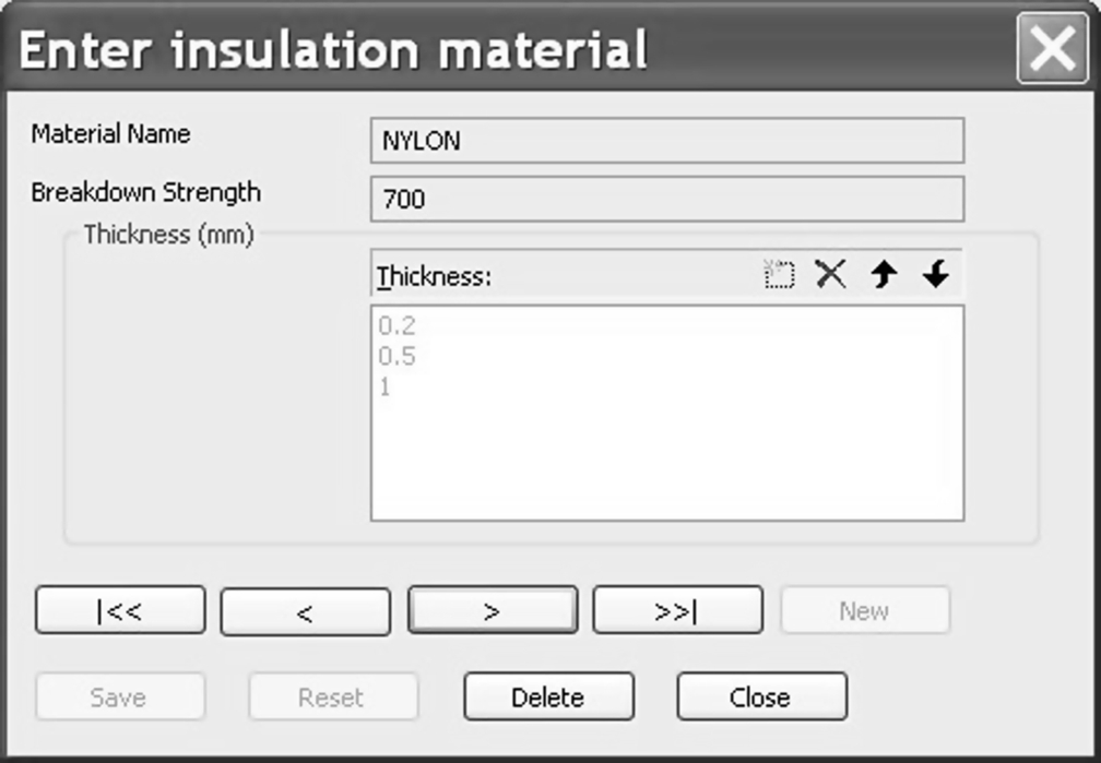
You can enter your own insulation materials: Tools > Data Entry > Insulation in the Enter insulation material window (Fig. 21.4).

Enter the design parameters as shown in Fig. 21.2 and click on Next >>.

Step 3: Electrical Parameters

This is where the electrical design parameters from the specifications are entered (Fig. 21.5).

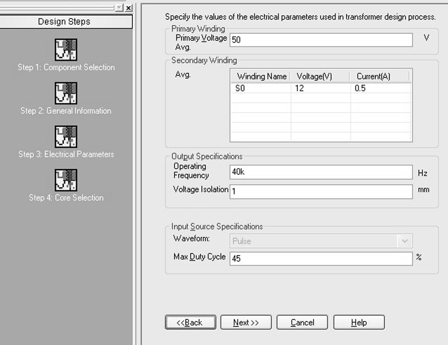
The secondary voltage and current are root mean square (RMS) values. The voltage isolation is the gap or distance between the primary and secondary windings.

Enter the electrical parameters as shown in Fig. 21.5 and click on Next >>.

Step 4: Core Selection

Selection of the magnetic core for the transformer depends on the shape and material. The physical diagram shown for the core in Fig. 21.6 is updated when you select another shape such as a toroid, EE or UU.

Change the Vendor name to Ferroxcube and from the Family Name pull-down menu, select Toroid and UU to view the respective geometrical data for the cores. Change the Family Name back to EE.

You can enter other manufacturer's core data by selecting Tools > Data Entry > Core Details > Core (Fig. 21.7).

You can also enter core material data by selecting Tools > Data Entry > Core Details > Material (Fig. 21.8).

Initially, you will specify a manufacturer's magnetic core material and then let MPE propose a magnetic core using the specified core material. The MPE will determine whether the coil windings will fit on the core.

The MPE core database includes the Ferroxcube range of magnetic cores. For this design, the Ferroxcube EE low-power (10 W) grade 3C81 material will be used as a starting point. These cores are specified for a 67 kHz switching frequency and an output voltage up to 12 V:

Set the Vendor Name to Ferroxcube.

Set the Family Name to EE.

Set the Material to 3C81.

Click on Propose Part.

The MPE will return a suitable Vendor Part and will show the respective physical dimensions for the core. The pull-down menu for Vendor Part contains a list of other suitable cores from the database that will also meet your specification.

In this example, the core E13_6_6 will have been selected, as shown in Fig. 21.9.

Click on Next >>.

Step 5: Bobbin-Winding Selection

This step selects the bobbin which fits on the core and on which the wire is wound. In Fig. 21.10, the Bobbin Part No. is shown as NO_NAME, which indicates that there are no bobbins in the MPE database. If no bobbin is specified, then a default bobbin wall thickness of 1 mm is used to calculate the bobbin dimensions based on the core dimensions. To create a new bobbin, select Tools > Data Entry > Core Details > Bobbin (Fig. 21.11).

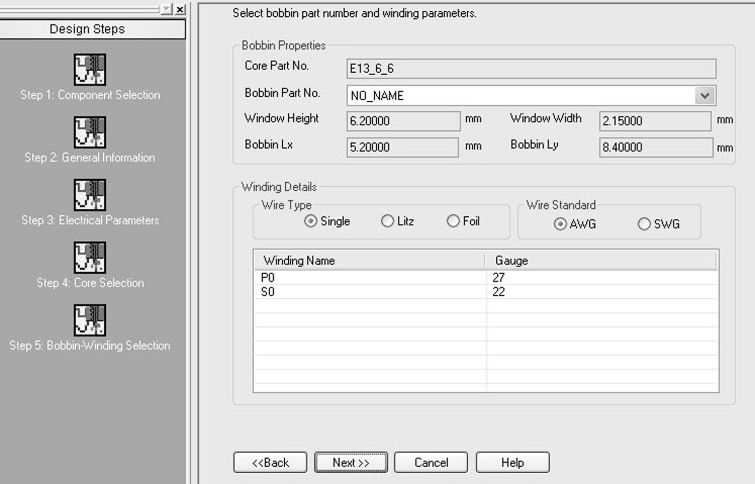
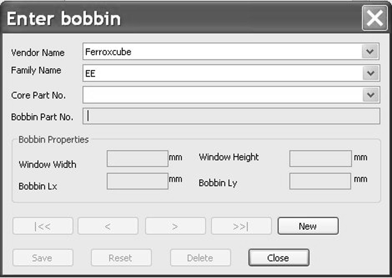
Fig. 21.12 shows the bobbin orientation and dimensions given in core vendor datasheets.

For the bobbin shown in Fig. 21.12, to fit into the core, the calculations are:

bobbin window height = core window height − (2 × bobbin thickness)

bobbin window width = core window width − (1 × bobbin thickness)

bobbin_Lx = core_Lx + (2 × bobbin thickness)

bobbin_Ly = core_Ly + (2 × bobbin thickness)

For this example, the default NO_NAME bobbin will be used, as the core dimensions are not yet finalized.

The Bobbin-Winding Selection window in Fig. 21.10 also shows the proposed wire types (diameters) for the primary and secondary coils. You can also select between the different AWG and SWG wire standards.

Click on Next >>.

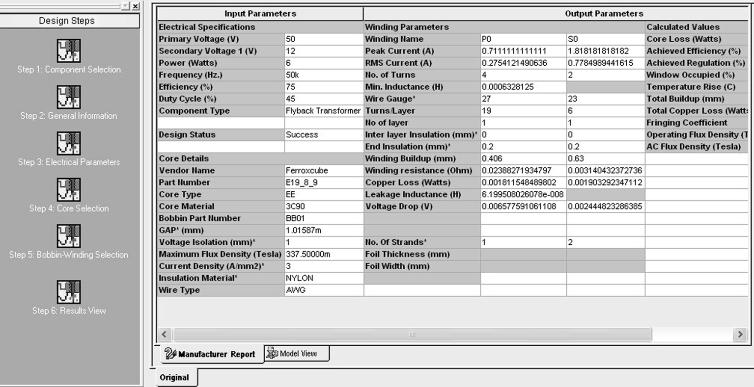
Step 6: Results View

Fig. 21.13 shows the spreadsheet of results. In order to see the full spreadsheet, turn off the Steps view: View > Steps View.

In the spreadsheet, the Design Status reports that there is an error (Fig. 21.14) and the warning message at the bottom of the results spreadsheet indicates that the P0 winding could not fit into the core.

So either the wire diameter for the secondary needs to be reduced or you need to use a different core material or a larger core. You could also reduce the distance between the primary and secondary windings (Voltage isolation in Step 3).

Go back to Step 4: Core selection and select the material as 3C90.

Click on Propose Part.

Select the E19_8_9 core, which has a larger core size, as seen in Fig. 21.15.

Click on Next >> and progress to the Results View.

You should see the Design Status reporting Success (Fig. 21.16).

Now you need to create the bobbin which will fit in the core and run the calculations again.

Go back to the Core selection (Step 4) and select Tools > Data Entry > Core Details > Bobbin as shown in Fig. 21.17. Select the proposed part, which was the Ferroxcube, EE core 19_8_9. Enter a suitable Bobbin Part No., for example BB01.

The core winding area dimensions given in Fig. as 21.15 are shown again in Fig. 21.17.

Referencing Fig. 21.12 and the associated calculations and using a bobbin wall thickness of 1 mm, the required bobbin dimensions are given as:

bobbin window height = 11.38 − 2 = 9.39 mm

bobbin window width = 4.79 − 1 = 3.79 mm

bobbin_Lx = 4.75 + 2 = 6.75 mm

bobbin_Ly = 8.71 + 2 = 10.71 mm

Go back to Step 5 (Bobbin-winding selection) and select Tools > Data Entry > Core Details Bobbin. Name the Bobbin BB01, enter the Bobbin data as shown in Fig. 21.18 and click on Save.

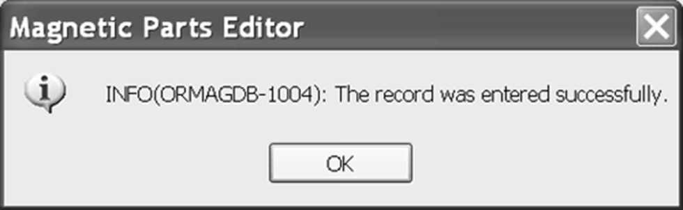
When you save the new bobbin, a message will appear informing you that the record was entered successfully into the database. Click on OK.

Proceed to Step 6 and check that the Design Status is still showing Success.

Save the design, which will generate a flyback .mgd file.

When you save the design, a PSpice model will be created. In this example the flyback.lib file will be created. By selecting the Model View tab at the bottom of the Results Spreadsheet, you can view the PSpice transformer model as shown in Fig. 21.19.

For the flyback topology, the transformer is modeled as a subcircuit with four terminals, V_IN1, V_IN2, V_OUT11 and V_OUT12. The transformer circuit representation is shown in Fig. 21.20.

With the Model View open, click on Save again to save the PSpice model.

Using the Model Editor Wizard in the Model Editor, a Capture part can be generated and associated to a transformer symbol as described in Chapter 16.

1. Open the PSpice Model Editor from the Start menu.
Start > All Programs > Cadence (or OrCAD) > PSpice > Simulation Accessories > Model Editor

2. In the Model Editor, select, File > New.

3. Select File > Model Import Wizard.

4. In the Specify Library window (Fig. 21.21), browse to the flyback.lib, accept the Destination Symbol Library as shown and click on Next >.

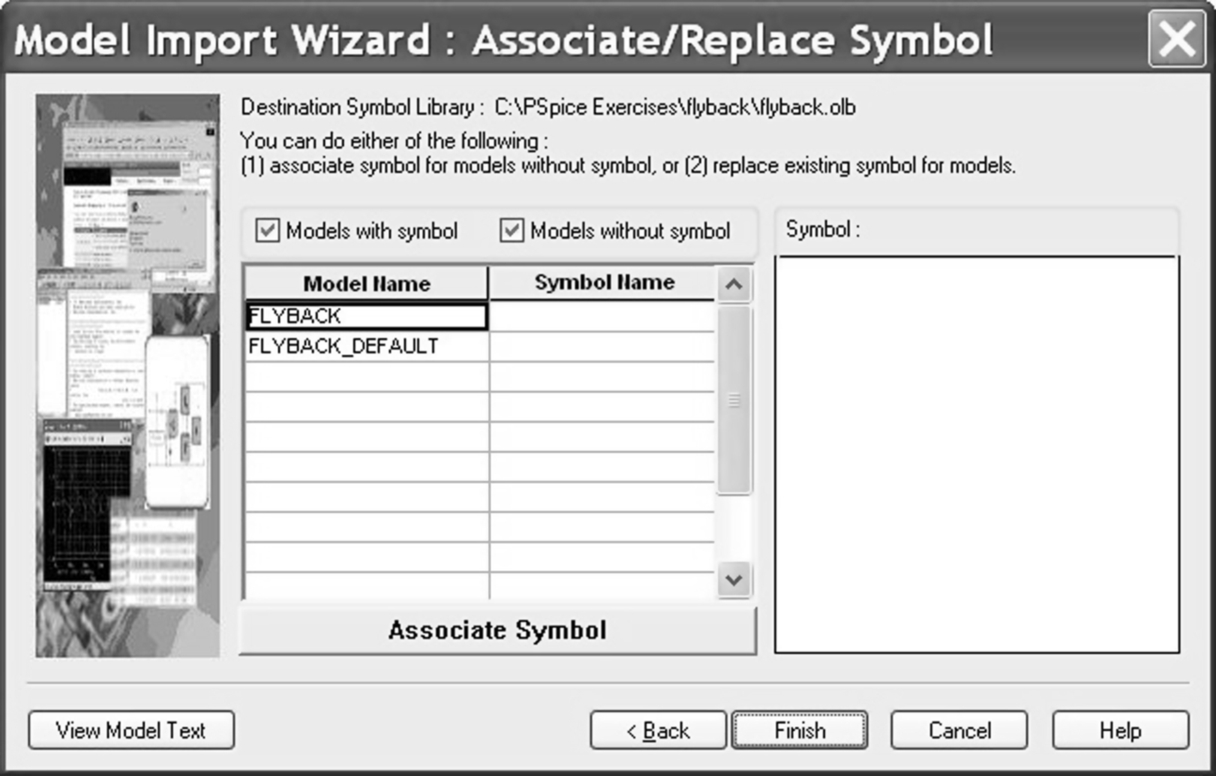
5. In the Associate/Replace Symbol window (Fig. 21.22), click on Associate Symbol. Select the Flyback model and click on Associate Symbol.

6. In the Select Matching window, click on the icon and select the breakout.olb library from the installed folder as < install path > OrCAD (or Cadence) > version xx.x > Tools > Capture > library > pspice > breakout.olb.

7. A list of matching symbols with the same number of pins as the flyback model has will be listed. Select the XFRM_NONLINEAR transformer as shown in Fig. 21.23 and click on Next >.

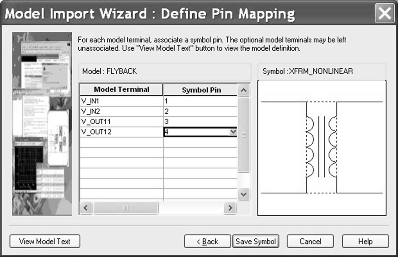
8. You have to associate the symbol pins with the model terminals. Select the pins as shown in Fig. 21.24 and then click on Save Symbol. The pins are in the same order as for the subcircuit model (Fig. 21.19).

9. You should see the model name shown with an associated symbol (Fig. 21.25).

10. Click on Finish and click on No in the sch2cap window. Check there are no error messages in the Summary Status window and click on OK. The Capture part and model are ready to be used.