The most relevant render parameters when dealing with time-dependent things are the current frame number and the frame rate (the number of frames per second). These parameters are provided grouped together as a rendering context by the Scene module, most via function calls, some as variables:

scn = Scene.GetCurrent()
context = scn.getRenderingContext()
current_frame = context.currentFrame()
start_frame = context.startFrame()
end_frame = context.endFrame()
frames_per_second = context.fps

With this information we can now calculate the time, either absolute or relative to the start frame:

absolute_time = current_frame/float(frames_per_second)
relative_time = (current_frame-start_frame)/float(frames_per_second)

Note the conversion to float in the denominator (highlighted). That way we ensure that the division is treated as a floating point operation. This is not strictly necessary since fps is returned as a float but many people assume the frame rate to be some integer value such as 25 or 30. This is, however, not always the case (for example, NTSC encoding uses a fractional frame rate) so we better make this explicit. Also note that we cannot do away with this division, otherwise when people would change their mind about their chosen frame rate the speed of the animation would change.

Accurately simulating the look of ripples caused by falling droplets may seem difficult but is straightforward, albeit a bit involved. Readers interested in the underlying mathematics might want to check some reference (for example http://en.wikipedia.org/wiki/Wave). Our goal, however, is not to simulate the real world as accurately as possible but to provide the artist with a texture that looks good and is controllable so that the texture may even be applied in situations which are not realistic.

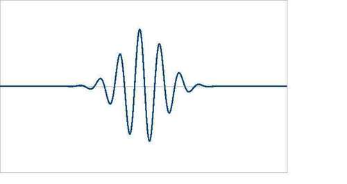
So instead of making the speed at which the ripple travels dependent on things, such as the viscosity of the water, we provide speed as a tunable input to our Pynode. Likewise for the height and width of the ripple and the rate at which the height of the ripple diminishes as it expands. Basically, we approximate our little packet of ripples as it radiates outward from the point of impact of a droplet by a cosine function multiplied by an exponential function and a damping factor. This may sound dangerously like mathematics again, but it can be easily visualized:

To calculate the height at any position x, y in our texture the above can be implemented as follows:

position_of_maximum=speed*time
damping = 1.0/(1.0+dampf*position_of_maximum)
distance = sqrt((x-dropx)**2+(y-dropy)**2)
height = damping*a*exp(-(distance-position_of_maximum)**2/c)*  cos(freq*(distance-position_of_maximum))

Here, dropx and dropy are the positions of impact of a drop and a is our tunable height parameter.

The effects of more drops dropped at different times and at different locations may simply be calculated by summing the resulting heights.

A single drop is not rain of course, so we would like to see the effects of many random drops added together. Therefore, we have to choose random impact locations and times for as many droplets as we'd like to simulate.

We would have to do this every time a call to the __call__() method is made (this is, for every visible pixel in our texture). However, this would be a tremendous waste of processing power because calculating many random numbers and allocating and releasing memory for possibly a large number of drops is expensive.

Fortunately, we can store these results as instance variables of our Pynode. Of course, we should be careful to check that no input parameters have changed between invocations of __call__() and take appropriate action if they have changed. The general pattern would look like this:

class MyNode(Node.Scripted):
def __init__(self, sockets):
sockets.input = [Node.Socket('InputParam', val = 1.0)]
sockets.output = [Node.Socket('OutputVal' , val = 1.0)]
self.InputParam = None
self.Result = None
def __call__(self):
if self.InputParam == None or 
self.InputParam != self.input.InputParam :
self.InputParam = self.input.InputParam
self.Result = expensive_calculation ...
self.output.OutputVal = other_calculations_using_Result …

This pattern works only if the input parameter changes infrequently, for example, only if the user changes it. If the input changes every pixel because the input socket is connected to the output of another node—the suggested scheme only costs time instead of saving some.

Our goal is to generate a ripple pattern that can be used as a normal. so we need some way to derive the normal from the calculated heights. Blender does not provide us with such a conversion node for materials so we have to devise a scheme ourselves.

Now, as in the case of ripples, we could, in principle, calculate an exact normal for our rain drops as well, but instead of going the mathematical way again we adapt a method used by many built-in noise textures to calculate the normal that works irrespective of the underlying function.

As long as we can evaluate a function at three points: f(x,y),f(x+nabla,y), and f(x,y+nabla) we can estimate the direction of the normal at x,y by looking at the slopes of our function in the x and y direction. The surface normal will be the unit vector perpendicular to the plane defined by these two slopes. We can take any small value for nabla to start and if it doesn't look good, we can make it smaller.

Taking all of these ideas from the preceding paragraphs, we can cook up the following code for our raindrops Pynode (with import statements omitted):

class Raindrops(Node.Scripted):
def __init__(self, sockets):
sockets.input = [Node.Socket('Drops_per_second' , val = 5.0, min = 0.01, max = 100.0),
Node.Socket('a',val=5.0,min=0.01,max=100.0),
Node.Socket('c',val=0.04,min=0.001,max=10.0),
Node.Socket('speed',val=1.0,min=0.001, max=10.0),
Node.Socket('freq',val=25.0,min=0.1, max=100.0),
Node.Socket('dampf',val=1.0,min=0.01, max=100.0),
Node.Socket('Coords', val = 3*[1.0])]
sockets.output = [Node.Socket('Height', val = 1.0),
Node.Socket('Normal', val = 3 *[0.0])]
self.drops_per_second = None
self.ndrops = None

The initialization code defines a number of input sockets besides the coordinates. Drops_per_second should be self explanatory. a and c are the overall height and width of the ripples traveling outward from the point of impact. speed and freq determine how fast our ripples travel and how close ripples are together. How fast the height of the ripples diminishes as they travel outward is determined by dampf.

We also define two output sockets: Height will contain the calculated height and Normal will contain the corresponding normal at that same point. The Normal is what you would normally use to obtain the rippling surface effect, but the calculated height might be useful for example to attenuate the reflectance value of the surface.

The initialization ends with the definition of some instance variables that will be used to determine if we need to calculate the position of the drop impacts again as we will see in the definition of the __call__() function.

The definition of the __call__() function starts off with the initialization of a number of local variables. One notable point is that we set the random seed used by the functions of the Noise module (highlighted in the following code). In this way, we make sure that each time we recalculate the points of impact we get repeatable results, that is if we set the number of drops per second first to ten, later to twenty, and then back to ten, the generated pattern will be the same. If you would like to change this you could add an extra input socket to be used as input for the setRandomSeed() function:

def __call__(self):
twopi = 2*pi
col = [0,0,0,1]
nor = [0,0,1]
tex_coord = self.input.Coords
x = tex_coord[0]
y = tex_coord[1]
a = self.input.a
c = self.input.c
Noise.setRandomSeed(42)

scn = Scene.GetCurrent()
context = scn.getRenderingContext()
current_frame = context.currentFrame()
start_frame = context.startFrame()
end_frame = context.endFrame()
frames_per_second = context.fps
time = current_frame/float(frames_per_second)

The next step is to determine whether we have to calculate the positions of the points of impact of the drops anew. This is necessary only when the value of the input socket Drops_per_second is changed by the user (you could hook up this input to some other node that changes this value at every pixel, but that wouldn't be a good idea) or when the start or stop frame of the animation changes, as this influences the number of drops we have to calculate. This test is performed in the highlighted line of the following code by comparing the newly obtained values to the ones stored in the instance variables:

drops_per_second = self.input.Drops_per_second
# calculate the number of drops to generate
# in the animated timeframe
ndrops = 1 + int(drops_per_second * (float(end_frame)
start_frame+1)/frames_per_second )
if self.drops_per_second != drops_per_second
or self.ndrops != ndrops:
self.drop = [ (Noise.random(), Noise.random(),
Noise.random() + 0.5) for i in range(ndrops)]
self.drops_per_second = drops_per_second
self.ndrops = ndrops

If we do have to calculate the position of the drops anew we assign a list of tuples to the self.drop instance variable, each consisting of the x and y position of the drop and a random drop size that will attenuate the height of the ripples.

The rest of the lines are all executed each time __call__() is called but the highlighted line does show a significant optimization. Because drops that have not yet fallen in the current frame do not contribute to the height, we exclude those from the calculation:

speed=self.input.speed
freq=self.input.freq
dampf=self.input.dampf
height = 0.0
height_dx = 0.0
height_dy = 0.0
nabla = 0.01
for i in range(1+int(drops_per_second*time)):
dropx,dropy,dropsize = self.drop[i]
position_of_maximum=speed*time-i/float(drops_per_second)
damping = 1.0/(1.0+dampf*position_of_maximum)
distance = sqrt((x-dropx)**2+(y-dropy)**2)
height += damping*a*dropsize*
exp(-(distance-position_of_maximum)**2/c)*
cos(freq*(distance-position_of_maximum))
distance_dx = sqrt((x+nabla-dropx)**2+(y-dropy)**2)
height_dx += damping*a*dropsize*
exp(-(distance_dx-position_of_maximum)**2/c)*
cos(freq*(distance_dx-position_of_maximum))
distance_dy = sqrt((x-dropx)**2+(y+nabla-dropy)**2)
height_dy += damping*a*dropsize*
exp(-(distance_dy-position_of_maximum)**2/c)*
cos(freq*(distance_dy-position_of_maximum))

In the preceding code we actually calculate the height at three different positions to be able to approximate the normal (as explained previously). These values are used in the following lines to determine the x and y components of the normal (the z component is set to one). The calculated height itself is divided by the number of drops (so the average height will not change when the number of drops is changed) and by the overall scaling factor a, which may be set by the user before it is assigned to the output socket (highlighted):

nor[0]=height-height_dx
nor[1]=height-height_dy
height /= ndrops * a
self.output.Height = height
N = (vec(self.shi.surfaceNormal)+0.2*vec(nor)).normalize()
self.output.Normal= N
__node__ = Raindrops

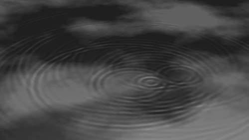
The calculated normal is then added to the surface normal at the pixel where we are calculating so the ripples will still look good on a curved surface and normalized before assigning it to the output socket. The final line as usual defines a meaningful name for this Pynode. The full code and a sample node setup are available as raindrops.py in raindrops.blend. A sample frame from an animation is shown in the next screenshot:

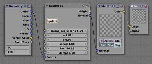
A sample node setup is shown in the following screenshot: