15.1 Introduction

We have seen how objects having quite simple shapes may be located in digital images via the Hough transform. For more complex shapes this approach tends to require excessive computation. In general, this problem may be overcome by locating objects from their features. Suitable salient features include small holes, corners, straight, circular, or elliptical segments, and any readily localizable subpatterns. Earlier chapters have shown how such features may be located. However, at some stage it becomes necessary to find methods for collating the information from the various features in order to recognize and locate the objects containing them. This task is studied in the present chapter.

It is perhaps easiest to envisage the feature collation problem when the features themselves are unstructured points carrying no directional information—nor indeed any attributes other than their x, y coordinates in the image. Then the object recognition task is often called point pattern matching.¹ The features that are closest to unstructured points are small holes, such as the “docker” holes in many types of biscuits. Corners can also be considered as points if their other attributes—including sharpness, and orientation—are ignored. In the following section we start with point features, and then we see how the attributes of more complex types of features can be included in recognition schemes.

Overall, we should remember that it is highly efficient to use small high-contrast features for object detection, since the computation involved in searching an image decreases as the template becomes smaller. As will be clear from the preceding chapters, the main disadvantage of such an approach to object detection is the loss in sensitivity (in a signal-to-noise sense) owing to the greatly impoverished information content of the point feature image. However, even the task of identifying objects from a rather small number of point features is far from trivial and frequently involves considerable computation, as we will see in this chapter. We start by studying a graph-theoretic approach to point pattern matching, which involves the “maximal clique” concept.

15.2 A Graph-theoretic Approach to Object Location

This section considers a commonly occurring situation that involves considerable constraints—objects appearing on a horizontal worktable or conveyor at a known distance from the camera. It is also assumed (1) that objects are flat or can appear in only a restricted number of stances in three dimensions, (2) that objects are viewed from directly overhead, and (3) that perspective distortions are small. In such situations, the objects may in principle be identified and located with the aid of very few point features. Because such features are taken to have no structure of their own, it will be impossible to locate an object uniquely from a single feature, although positive identification and location would be possible using two features if these were distinguishable and if their distance apart were known. For truly indistinguishable point features, an ambiguity remains for all objects not possessing 180° rotation symmetry. Hence, at least three point features are in general required to locate and identify objects at a known range. Clearly, noise and other artifacts such as occlusions modify this conclusion. When matching a template of the points in an idealized object with the points present in a real image, we may find the following:

These problems mean that we should in general be attempting to match a subset of the points in the idealized template to various subsets of the points in the image. If the point sets are considered to constitute graphs with the point features as nodes, the task devolves into the mathematical problem of subgraph—subgraph isomorphism, that is, finding which subgraphs in the image graph are isomorphic² to subgraphs of the idealized template graph. Of course, there may be a large number of matches involving rather few points. These would arise from sets of features that happen (see, for example, item (2) above) to lie at valid distances apart in the original image. The most significant matches will involve a fair number of features and will lead to correct object identification and location. A point feature matching scheme will be most successful if it finds the most likely interpretation by searching for solutions with the greatest internal consistency—that is, with the greatest number of point matches per object.

Unfortunately, the scheme of things presented here is still too simplistic in many applications, for it is insufficiently robust against distortions. In particular, optical (e.g., perspective) distortions may arise, or the objects themselves may be distorted, or by resting partly on other objects they may not be quite in the assumed stance. Hence, distances between features may not be exactly as expected. These factors mean that some tolerance has to be accepted in the distances between pairs of features, and it is common to employ a threshold such that interfeature distances have to agree within this tolerance before matches are accepted as potentially valid. Distortions produce more strain on the point matching technique and make it all the more necessary to seek solutions with the greatest possible internal consistency. Thus, as many features as possible should be taken into account in locating and identifying objects. The maximal clique approach is intended to achieve this.

As a start, as many features as possible are identified in the original image, and these are numbered in some convenient order such as the order of appearance in a normal TV raster scan. The numbers then have to be matched against the letters corresponding to the features on the idealized object. A systematic way to do this is to construct a match graph (or association graph) in which the nodes represent feature assignments and arcs joining nodes represent pairwise compatibilities between assignments. To find the best match, it is necessary to find regions of the match graph where the cross linkages are maximized. To do so, cliques are sought within the match graph. A clique is a complete subgraph—that is, one for which all pairs of nodes are connected by arcs. However, the previous arguments indicate that if one clique is completely included within another clique, the larger clique likely represents a better match—and indeed maximal cliques can be taken as leading to the most reliable matches between the observed image and the object model.

Figure 15.1a illustrates the situation for a general triangle: for simplicity, the figure takes the observed image to contain only one triangle and assumes that lengths match exactly and that no occlusions occur. The match graph in this example is shown in Fig. 15.1b. There are nine possible feature assignments, six valid compatibilities, and four maximal cliques, only the largest corresponding to an exact match.

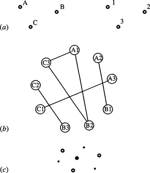
Figure 15.1 A simple matching problem—a general triangle: (a) basic labeling of model (left) and image (right); (b) match graph; (c) placement of votes in parameter space. In (b) the maximal cliques are: (1) A1, B2, C3; (2) A2, B1; (3) B3, C2; and (4) C1, A3. In (c) the following notation is used: , positions of observed features; •, positions of votes, position of main voting peak.

Figure 15.2a shows the situation for the less trivial case of a quadrilateral, the match graph being shown in Fig. 15.2b. In this case, there are 16 possible feature assignments, 12 valid compatibilities, and 7 maximal cliques. If occlusion of a feature occurs, this will (taken on its own) reduce the number of possible feature assignments and also the number of valid compatibilities. In addition, the number of maximal cliques and the size of the largest maximal clique will be reduced. On the other hand, noise or clutter can add erroneous features. If the latter are at arbitrary distances from existing features, then the number of possible feature assignments will be increased, but there will not be any more compatibilities in the match graph. The match graph will therefore have only trivial additional complexity. However, if the extra features appear at allowed distances from existing features, this will introduce extra compatibilities into the match graph and make it more tedious to analyze. In the case shown in Fig. 15.3, both types of complications—an occlusion and an additional feature—arise. There are now eight pairwise assignments and six maximal cliques, rather fewer overall than in the original case of Fig. 15.2. However, the important factors are that the largest maximal clique still indicates the most likely interpretation of the image and that the technique is inherently highly robust.

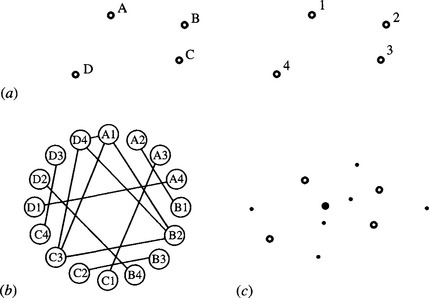
Figure 15.2 Another matching problem—a general quadrilateral: (a) basic labeling of model (left) and image (right); (b) match graph; (c) placement of votes in parameter space (notation as in Fig. 15.1).

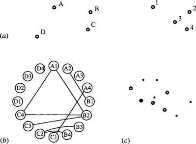
Figure 15.3 Matching when one feature is occluded and another is added: (a) basic labeling of model (left) and image (right); (b) match graph; (c) placement of votes in parameter space (notation as in Fig. 15.1).

When using methods such as the maximal clique approach, which involves repetitive operations, it is useful to look for a means of saving computation. When the objects being sought possess some symmetry, economies can be made. Consider the case of a parallelogram (Fig. 15.4). Here the match graph has 20 valid compatibilities, and there are 10 maximal cliques. Of these cliques, the largest two have equal numbers of nodes, and both identify the parallelogram within a symmetry operation. This means that the maximal clique approach is doing more computation than absolutely necessary. This can be avoided by producing a new “symmetry-reduced” match graph after relabeling the model template in accordance with the symmetry operations (see Fig. 15.5). This gives a much smaller match graph with half the number of pairwise compatibilities and half the number of maximal cliques. In particular, there is only one nontrivial maximal clique. Note, however, that the application of symmetry does not reduce its size.

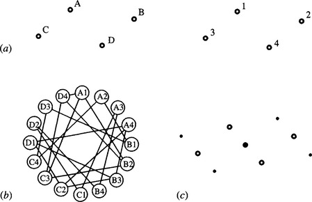
Figure 15.4 Matching a figure possessing some symmetry: (a) basic labeling of model (left) and image (right); (b) match graph; (c) placement of votes in parameter space (notation as in Fig. 15.1).

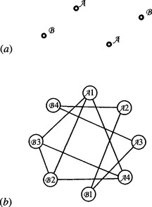
Figure 15.5 Using a symmetry-reduced match graph: (a) relabeled model template; (b) symmetry-reduced match graph.

15.2.1 A Practical Example—Locating Cream Biscuits

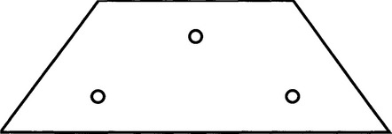
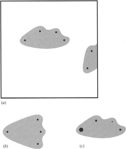
Figure 15.6a shows one of a pair of cream biscuits that are to be located from their “docker” holes. This strategy is advantageous because it has the potential for highly accurate product location prior to detailed inspection. (In this case, the purpose is to locate the biscuits accurately from the holes, and then to check the alignment of the biscuit wafers and detect any excess cream around the sides of the product.) The holes found by a simple template matching routine are indicated in Fig. 15.6b. The template used is rather small, and, as a result, the routine is fairly fast but fails to locate all holes. In addition, it can give false alarms. Hence, an “intelligent” algorithm must be used to analyze the hole location data.

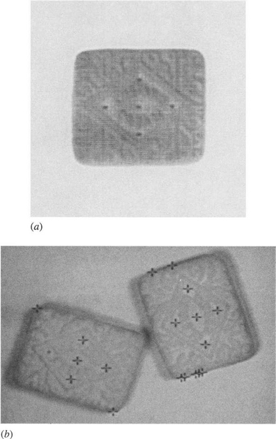
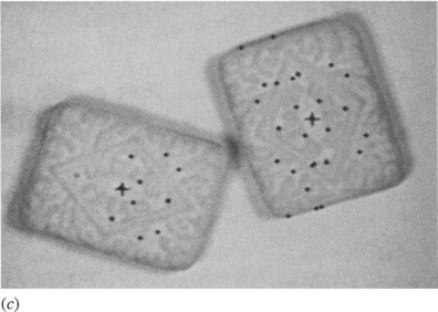
Figure 15.6 (a) A typical cream sandwich biscuit; (b) a pair of cream sandwich biscuits with crosses indicating the result of applying a simple hole detection routine; (c) the two biscuits reliably located by the GHT from the hole data in (b). The isolated small crosses indicate the positions of single votes.

This is a highly symmetrical type of object, and so it should be beneficial to employ the symmetry-reduced match graph described above. To proceed, it is helpful to tabulate the distances between all pairs of holes in the object model (Fig. 15.7b). Then this table can be regrouped to take account of symmetry operations (Fig. 15.7d). This will help when we come to build the match graph for a particular image. Analysis of the data in the above example shows that there are two nontrivial maximal cliques, each corresponding correctly to one of the two biscuits in the image. Note, however, that the reduced match graph does not give a complete interpretation of the image. It locates the two objects, but it does not confirm uniquely which hole is which.

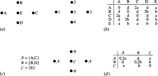
Figure 15.7 Interfeature distances for holes on cream biscuits: (a) basic labeling of model (left) and image (right); (b) allowed distance values; (c) revised labeling of model using symmetrical set notation; (d) allowed distance values. The cases of zero interfeature distance in the final table can be ignored as they do not lead to useful matches.

In particular, for a given starting hole of type A, it is not known which is which of the two holes of type B. This can be ascertained by applying simple geometry to the coordinates in order to determine, say, which hole of type B is reached by moving around the center hole E in a clockwise sense.

15.3 Possibilities for Saving Computation

In these examples, it is simple to check which subgraphs are maximal cliques. However, in real matching tasks it can quickly become unmanageable. (The reader is encouraged to draw the match graph for an image containing two objects of seven points!)

Figure 15.8 shows what is perhaps the most obvious type of algorithm for finding maximal cliques. It operates by examining in turn all cliques of a given number of nodes and finding what cliques can be constructed from them by adding additional nodes (bearing in mind that any additional nodes must be compatible with all existing nodes in the clique). This permits all cliques in the match graph to be identified. However, an additional step is needed to eliminate (or relabel) all cliques that are included as subgraphs of a new larger clique before it is known which cliques are maximal.

Figure 15.8 A simple maximal clique algorithm.

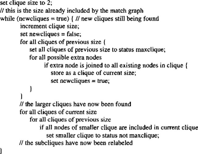
In view of the evident importance of finding maximal cliques, many algorithms have been devised for the purpose. The best of these is probably now close to the fastest possible speed of operation. Unfortunately, the optimum execution time is known to be bounded not by a polynomial in M (for a match graph containing maximal cliques of up to M nodes) but by a much faster varying function. Specifically, the task of finding maximal cliques is akin to the well-known traveling salesperson problem and is known to be NP-complete, implying that it runs in exponential time (see Section 15.4.1). Thus, whatever the run-time is for values of M up to about 6, it will typically be 100 times slower for values of M up to about 12 and 100 times slower again for M greater than ~15. In practical situations, this problem can be tackled in several ways:

Of these methods, the first should be used wherever applicable. Methods (2)-(4) amount to improving the implementation and are subject to diminishing returns. It should be noted that the execution time varies so rapidly with M that even the best software implementations are unlikely to give a practical increase in M of more than 2 (i.e., M → M + 2). Similarly, dedicated hardware implementations may only give increases in M of the order of 4 to 6. Method (5) is a “shortcut” approach that proves highly effective in practice. The idea is to search for specific subsets of the features of an object and then to hypothesize that the object exists and go back to the original image to check that it is actually present. Bolles and Cain (1982) devised this method when looking for hinges in quite complex images. In principle, the method has the disadvantage that the particular subset of an object that is chosen as a cue may be missing because of occlusion or some other artifact. Hence, it may be necessary to look for several such cues on each object. This is an example of further deviation from the matched filter paradigm, which reduces detection sensitivity yet again. The method is called the local-feature-focus (LFF) method because objects are sought by cues or local foci.

The maximal clique approach is a type of exhaustive search procedure and is effectively a parallel algorithm. This has the effect of making it highly robust but is also the source of its slow speed. An alternative is to perform some sort of sequential search for objects, stopping when sufficient confidence is attained in the interpretation or partial interpretation of the image. For example, the search process may be terminated when a match has been obtained for a certain minimum number of features on a given number of objects. Such an approach may be useful in some applications and will generally be considerably faster than the full maximal clique procedure when M is greater than about 6. Ullmann (1976) carried out an analysis of several tree-search algorithms for subgraph isomorphism in which he tested algorithms using artificially generated data; it is not clear how they relate to real images. The success or otherwise of all nonexhaustive search algorithms must, however, depend critically on the particular types of image data being analyzed. Hence, it is difficult to give further general guidance on this matter (but see Section 15.7 for additional comments on search procedures).

The final method listed above is based on the GHT. In many ways, this provides an ideal solution to the problem because it presents an exhaustive search technique that is essentially equivalent to the maximal clique approach, while not falling into the NP-complete category. This may seem contradictory, since any approach to a well-defined mathematical problem should be subject to the mathematical constraints known to be involved in its solution. However, although the abstract maximal clique problem is known to be NP-complete, the subset of maximal clique problems that arises from 2-D image-based data may well be solved with less computation by other means, and in particular by a 2-D technique. This special circumstance does appear to be valid, but unfortunately it offers no possibility of solving general NP-complete problems by reference to the specific solutions found using the GHT approach! The GHT approach is described in the following section.

15.4 Using the Generalized Hough Transform for Feature Collation

The GHT can be used as an alternative to the maximal clique approach, to collate information from point features in order to find objects. Initially, we consider situations where objects have no symmetries—as for the cases of Figs. 15.1–15.3.

To apply the GHT, we first list all features and then accumulate votes in parameter space at every possible position of a localization point L consistent with each pair of features (Fig. 15.9). This strategy is particularly suitable in the present context, for it corresponds to the pairwise assignments used in the maximal clique method. To proceed it is necessary merely to use the interfeature distance as a lookup parameter in the GHT R-table. For indistinguishable point features this means that there must be two entries for the position of L for each value of the interfeature distance. Note that we have assumed that no symmetries exist and that all pairs of features have different interfeature distances. If this were not so, then more than two vectors would have to be stored in the R-table per interfeature distance value.

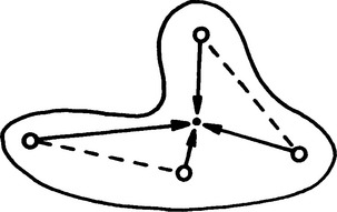
Figure 15.9 Method for locating L from pairs of feature positions. Each pair of feature points gives two possible voting positions in parameter space, when objects have no symmetries. When symmetries are present, certain pairs of features may give rise to up to four voting positions. This is confirmed on careful examination of Fig. 15.6c.

To illustrate the procedure, it is applied first to the triangle example of Fig. 15.1. Figure 15.1c shows the positions at which votes are accumulated in parameter space. There are four peaks with heights of 3, 1, 1, 1; it is clear that, in the absence of complicating occlusions and defects, the object is locatable at the peak of maximum size. Next, the method is applied to the general quadrilateral example of Fig. 15.2: this leads to seven peaks in parameter space, whose sizes are 6, 1, 1, 1, 1, 1, 1 (Fig. 15.2c).

Close examination of Figs. 15.1–15.3 indicates that every peak in parameter space corresponds to a maximal clique in the match graph. Indeed, there is a one-to-one relation between the two. In the uncomplicated situation being examined here, this is bound to be so for any general arrangement of features within an object, since every pairwise compatibility between features corresponds to two potential object locations, one correct and one that can be correct only from the point of view of that pair of features. Hence, the correct locations all add to give a large maximal clique and a large peak in parameter space, whereas the incorrect ones give maximal cliques, each containing two wrong assignments and each corresponding to a false peak of size 1 in parameter space. This situation still applies even when occlusions occur or additional features are present (see Fig. 15.3). The situation is slightly more complicated when symmetries are present, with each of the two methods deviating in a different way. Space does not permit the matter to be explored in depth here, but the solution for the case of Fig. 15.4a is presented in Fig. 15.4c. Overall, it seems simplest to assume that there is still a one-to-one relationship between the solutions from the two approaches.

Finally, consider again the example of Section 15.2.1 (Fig. 15.6a), this time obtaining a solution by the GHT. Figure 15.6c shows the positions of candidate object centers as found by the GHT. The small isolated crosses indicate the positions of single votes, and those very close to the two large crosses lead to voting peaks of weights 10 and 6 at these respective positions. Hence, object location is both accurate and robust, as required.

15.5 Generalizing the Maximal Clique and Other Approaches

This section considers how the graph matching concept can be generalized to cover alternative types of features and various attributes of features. We restricted our earlier discussion to point features and in particular to small holes that were supposed to be isotropic. Corners were also taken as point features by ignoring attributes other than position coordinates. Both holes and corners seem to be ideal in that they give maximum localization and hence maximum accuracy for object location. Straight lines and straight edges at first appear to be rather less well suited to the task. However, more careful thought shows that this is not so. One possibility is to use straight lines to deduce the positions of corners that can then be used as point features, although this approach is not as powerful as might be hoped because of the abundance of irrelevant line crossings that are thrown up. (In this context, note that the maximal clique method is inherently capable of sorting the true corners from the false alarms.) A more elegant solution is simply to determine the angles between pairs of lines, referring to a lookup table for each type of object to determine whether each pair of lines should be marked as compatible in the match graph. Once the match graph has been built, an optimal match can be found as before (although ambiguities of scale will arise which will have to be resolved by further processing). These possibilities significantly generalize the ideas of the foregoing sections.

Other types of features generally have more than two specifying parameters, one of which may be contrast and the other size. This applies for most holes and circular objects, although for the smallest (i.e., barely resolvable) holes it is sometimes most practicable to take the central dip in intensity as the measured parameter. For straight lines the relevant size parameter is the length. (We here count the line ends, if visible, as points that will already have been taken into account.) Corners may have a number of attributes, including contrast, color, sharpness, and orientation—none of which is likely to be known with high accuracy. Finally, more complex shapes such as ellipses have orientation, size, and eccentricity, and again contrast or color may be a usable attribute. (Generally, contrast is an unreliable measure because of possible variations in the background.)

So much information is available that we need to consider how best to use it for locating objects. For convenience this is discussed in relation to the maximal clique method. Actually, the answer is very simple. When compatibilities are being considered and the arcs are being drawn in the match graph, any available information may be taken into account in deciding whether a pair of features in the image matches a pair of features in the object model. In Section 15.2 the discussion was simplified by taking interfeature distances as the only relevant measurements. However, it is quite acceptable to describe the features in the object model more fully and to insist that they all match within prespecified tolerances. For example, holes and corners may be permitted to lead to a match only if the holes are of the correct size, the corners are of the correct sharpness and orientation, and the distances between these features are also appropriate. All relevant information has to be held in suitable lookup tables. In general, the gains easily outweigh the losses, since a considerable number of potential interpretations will be eliminated—thereby making the match graph significantly simpler and reducing, in many cases by a large factor, the amount of computation that is required to find the maximal cliques. Note, however, that there is a limit to this, since in the absence of occlusions and erroneous tolerances on the additional attributes, the number of nodes in the match graph cannot be less than the square of the number of features in an object, and the number of nodes in a maximal clique will be unchanged.

Thus, extra feature attributes are of great value in reducing computation; they are also useful in making interpretation less ambiguous, a property that is “obvious” but not always realizable. In particular, extra attributes help in this way only if (1) some of the features on an object are missing, through occlusion or for other reasons such as breakage, or (2) the distance tolerances are so large as to make it unclear which features in the image match those in the model.

Suppose next that the distance attributes become very imprecise, either because of shape distortions or because of unforeseen rotations in 3-D. How far can we proceed under these circumstances? In the limit of low-distance accuracy, we may only be able to employ an “adjacent to” descriptor. This parallels the situation in general scene analysis, where use is made of a number of relational descriptors such as “on top of,” “to the left of,” and so on. Such possibilities are considered in the next section.

15.6 Relational Descriptors

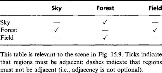
The previous section showed how additional attributes could be incorporated into the maximal clique formalism so that the effects of diminishing accuracy of distance measurement could be accommodated. This section considers what happens when the accuracy of distance measurement drops to zero and we are left just with relational attributes such as “adjacent to,” “near,” “inside,” “underneath,” “on top of,” and so on. We start by taking adjacency as the basic relational attribute. To illustrate the approach, imagine a simple outdoor scene where various rules apply to segmented regions. These rules will be of the type “sky may be adjacent to forest,” “forest may be adjacent to field,” and so on. Note that “adjacent to” is not transitive; that is, if P is adjacent to Q, and Q is adjacent to R, this does not imply that P is adjacent to R. (In fact, it is quite likely that P will not be adjacent to R, for Q may well separate the two regions completely!)

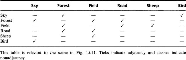
The rules for a particular type of scene may be summarized as in Table 15.1. Now consider the scene shown in Fig. 15.10. Applying the rules for adjacency from Table 15.1 will be seen to permit four different solutions, in which regions 1 to 3 may be interpreted as:

Table 15.1 Adjacency table for simple scene

Figure 15.10 Regions in a simple scene: 1, sky; 2, forest; 3, field.

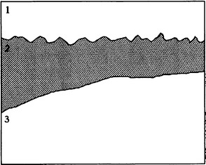
Evidently, there are too few constraints. Possible constraints are the following: sky is above field and forest, sky is blue, field is green, and so on. Of these, the first is a binary relation like adjacency, whereas the other two are unary constraints. It is easy to see that two such constraints are required to resolve completely the ambiguity in this particular example.

Paradoxically, adding further regions can make the situation inherently less ambiguous. This is because other regions are less likely to be adjacent to all the original regions and in addition may act in such a way as to label them uniquely. This is seen in Fig. 15.11, which is interpreted by reference to Table 15.2, although the keys to unique interpretation are the notions that any small white objects must be sheep,andany small dark objects must be birds. On analyzing the available data, the whole scene can now be interpreted unambiguously. As expected, the maximal clique technique can be applied successfully, although to achieve this, assignments must be taken to be compatible not only when image regions are adjacent and their interpretations are marked as adjacent, but also when image regions are nonadjacent and their interpretations are marked as nonadjacent. (The reason for this is easily seen by drawing an analogy between adjacency and distance, adjacent and nonadjacent corresponding, respectively, to zero and a significant distance apart.) Note that in this scene analysis type of situation, it is very tedious to apply the maximal clique method manually because there tend to be a fair number of trivial solutions (i.e., maximal cliques with just a few nodes).

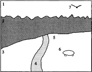
Figure 15.11 Regions in a more complex scene: 1, sky; 2, forest; 3, field; 4, road; 5, field; 6, sheep; _7bird

Table 15.2 Adjacency table for more complex scene

Perhaps oddly, some of the trivial solutions that the maximal clique technique gives rise to are provably incorrect. For example, in the above problem, one solution appears to include regions 1 and 2 being forest and sky, respectively, whereas it is clear from the presence of birds that region 1 cannot be forest and must be sky. Here logic appears to be a stronger arbiter of correctness than an evidence-building scheme such as the maximal clique technique. On the plus side, however, the maximal clique technique will take contradictory evidence and produce the best possible response. For example, if noise appears and introduces an invalid “bird” in the forest, it will simply ignore it, whereas a purely logic-based scheme will be unable to find a satisfactory solution. Clearly, much depends on the accuracy and universality of the assertions on which these schemes are based.

Logical problems such as the ones outlined here are commonly tackled with the aid of declarative languages such as PROLOG, in which the rules are written explicitly in a standard form not dissimilar to IF statements in English. Space does not permit a full discussion of PROLOG here. However, it should be noted that PROLOG is basically designed to obtain a single “logical” solution where one exists. It can also be instructed to search for all available solutions or for any given number of solutions. When instructed to search for all solutions, it will finally arrive at the same main set of solutions as the maximal clique approach (although, as indicated above, noise can make the situation more complicated). Thus, despite their apparent differences, these approaches are quite similar. It is the implementation of the underlying search problem that is different. (PROLOG uses a “depth-first” search strategy see below.) Next, we move on to another scheme—that of relaxation labeling—which has a quite different formulation.

Relaxation labeling is an iterative technique in which evidence is gradually built up for the proper labeling of the solution space—in this case, of the various regions in the scene. Two main possibilities exist. In the first, called discrete relaxation, evidence for pairs of labels is examined and a label discarding rule is instigated that eliminates at each iteration those pairs of labels that are currently inconsistent. This technique is applied until no further change in the labeling occurs. The second possibility is that of probabilistic relaxation. Here the labels are set up numerically to correspond to the probabilities of a given interpretation of each region; that is, a table is compiled of regions against possible interpretations, each entry being a number representing the probability of that particular interpretation. After providing a suitable set of starting probabilities (possibly all being weighted equally), these are updated iteratively, and in the ideal case they converge on the values 0 or 1 to give a unique interpretation of the scene. Unfortunately, convergence is by no means guaranteed and can depend on the starting probabilities and the updating rule. A prearranged constraint function defines the underlying process, and this could in principle be either better or worse at matching reality than (for example) the logic programming techniques that are used in PROLOG. Relaxation labeling is a complex optimization process and is not discussed further here. Suffice it to say that the technique often runs into problems of excessive computation. The reader is referred to the seminal paper by Rosenfeld et al. (1976) and other papers mentioned in Section 15.9 for further details.

15.7 Search

We have shown how the maximal clique approach may be used to locate objects in an image, or alternatively to label scenes according to predefined rules about what arrangements of regions are expected in scenes. In either case, the basic process being performed is that of a search for solutions that are compatible with the observed data. This search takes place in assignment space—that is, a space in which all combinations of assignments of observed features with possible interpretations exist. The problem is that of finding one or more valid sets of observed assignments.

Generally, the search space is very large, so that an exhaustive search for all solutions would involve enormous computational effort and would take considerable time. Unfortunately, one of the most obvious and appealing methods of obtaining solutions, the maximal clique approach, is NP-complete and can require impracticably large amounts of time to find all the solutions. It is therefore useful to clarify the nature of the maximal clique approach. To achieve this clarification, we first describe the two main categories of search—breadth-first and depth-first search.

Breadth-first search is a form of search that systematically works down a tree of possibilities, never taking shortcuts to nearby solutions. Depth-first search, in contrast, involves taking as direct a path as possible to individual solutions, stopping the process when a solution is found and backtracking up the tree whenever a wrong decision is found to have been made. It is normal to curtail the depth-first search when sufficient solutions have been found, and this means that much of the tree of possibilities will not have been explored. Although breadth-first search can be curtailed similarly when enough solutions have been found, the maximal clique approach as described earlier is in fact a form of breadth-first search that is exhaustive and runs to completion.

In addition to being an exhaustive breadth-first search, the maximal clique approach may be described as being “blind” and “flat”; that is, it involves neither heuristic nor hierarchical means of guiding the search. Faster search methods involve guiding the search in various ways. First, heuristics are used to specify at various stages in which direction to proceed (which node of the tree to expand) or which paths to ignore (which nodes to prune). Second, the search can be made more “hierarchical,” so that it searches first for outline features of a solution, returning later (perhaps in several stages) to fill in the details. Details of these techniques are omitted here. However, Rummel and Beutel (1984) used an interesting approach: they searched images for industrial components using features such as corners and holes, alternating at various stages between breadth-first and depth-first search by using a heuristic based on a dynamically adjusted parameter. This parameter was computed on the basis of how far the search was still away from its goal, and the quality of the fit when a “guide factor” based on the number of features required for recognition was adjusted. Rummel and Beutel noted the existence of a tradeoff between speed and accuracy. The problem was that trying to increase speed introduces some risk of not finding the optimum solution.

15.8 Concluding Remarks

In this chapter the maximal clique approach was seen to be capable of finding solutions to the task of recognizing objects from their features and the related task of scene analysis. Although ultimately these are search problems, a much greater range of methods is applicable to each. In particular, blind, flat, exhaustive breadth-first search (i.e., the maximal clique method) involves considerable computation and is often best replaced by guided depth-first search, with suitable heuristics being devised to guide the search. In addition, languages such as PROLOG can implement depth-first search and rather different procedural techniques such as relaxation labeling are available and should be considered (although these are subject to their own complexities and computational problems).

The task of recognizing objects from their features tends to involve considerable computation, and the GHT can provide a satisfactory solution to these problems. This is probably because the graph theory representation is not well matched to the relevant real-space template matching task in the way that the GHT is. Here, recall what was noted in Chapter 11—that the GHT is particularly well suited to object detection in real space as it is one type of spatial matched filter. Indeed, the maximal clique approach can be regarded as a rather inefficient substitute for the GHT form of the spatial matched filter. Furthermore, the LFF method takes a shortcut to save computation, which makes it less like a spatial matched filter, thereby adversely affecting its ability to detect objects among noise and clutter. Note that for scene analysis, where relational descriptors rather than precise dimensional (binary) attributes are involved, the GHT does not provide any very obvious possibilities—probably because we are dealing here with much more abstract data that are linked to real space only at a very high level (but see the work of Kasif et al., 1983).

Finally, note that, on an absolute scale, the graph matching approach takes very little note of detailed image structure, using at most only pairwise feature attributes. This is adequate for 2-D image interpretation but inadequate for situations such as 3-D image analysis where there are more degrees of freedom to contend with (normally three degrees of freedom for position and three for orientation, for each object in the scene). Hence, more specialized and complex approaches need to be taken in such cases; these approaches are examined in the following chapter.

15.9 Bibliographical and Historical Notes

Graph matching and clique finding algorithms started to appear in the literature around 1970; for an early solution to the graph isomorphism problem, see Corneil and Gottlieb (1970). The subgraph isomorphism problem was tackled soon after by Barrow et al. (1972; see also Ullmann, 1976). The double subgraph isomorphism (or subgraph-subgraph isomorphism) problem is commonly tackled by seeking maximal cliques in the match graph, and algorithms for achieving this have been described by Bron and Kerbosch (1973), Osteen and Tou (1973), and Ambler et al. (1975). (Note that in 1989 Kehtarnavaz and Mohan reported preferring the algorithm of Osteen and Tou on the grounds of speed.) Improved speed has also been achieved using the minimal match graph concept (Davies, 1991a).

Bolles (1979) applied the maximal clique technique to real-world problems (notably the location of engine covers) and showed how operation could be made more robust by taking additional features into account. By 1982, Bolles and Cain had formulated the local-feature-focus method, which (1) searches for restricted sets of features on an object, (2) takes symmetry into account to save computation, and (3) reconsiders the original image data in order to confirm a valid match. Bolles and Cain give various criteria for ensuring satisfactory solutions with this type of method.

Not satisfied by the speed of operation of maximal clique methods, other workers have tended to use depth-first search techniques. Rummel and Beutel (1984) developed the idea of alternating between depth-first and breadth-first searches as dictated by the data a powerful approach, although the heuristics they used may well lack generality. Meanwhile, Kasif et al. (1983) showed how a modified GHT (the “relational HT”) could be used for graph matching, although their paper gives few practical details. A somewhat different application of the GHT to perform 2-D matching (Davies, 1988g) was described in Section 15.4 and has been extended to optimize accuracy (Davies, 1992d) as well as to improve speed (Davies, 1993b). Geometric hashing has been developed to perform similar tasks on objects with complex polygonal shapes (Tsai, 1996).

Relaxation labeling in scenes dates from the seminal paper by Rosenfeld et al. (1976). For later work on relaxation labeling and its use for matching, see Kitchen and Rosenfeld (1979), Hummel and Zucker (1983), and Henderson (1984); for rule-based methods in image understanding, see, for example, Hwang et al. (1986); and for preparatory discussion and careful contrasting ofthese approaches, see Ballard and Brown (1982). Discussion of basic artificial intelligence search techniques and rule-based systems may be found in Charniak and McDermott (1985). A useful reference on PROLOG is Clocksin and Mellish (1984).

Over the past three decades, inexact matching algorithms have acquired increasing predominance over exact matching methods because of the ubiquitous presence of noise, distortions, and missing or added feature points, together with inaccuracies and thus mismatches of feature attributes. One class of work on inexact (or “error-tolerant”) matching considers how structural representations should be compared (Shapiro and Haralick, 1985). This early work on similarity measures shows how the concept of string edit distance can be applied to graphical structures (Sanfeliu and Fu, 1983). The formal concept of edit distance was later extended by Bunke and Shearer (1998) and Bunke (1999), who considered and rationalized the cost functions for methods such as graph isomorphisms, subgraph isomorphisms, and maximum common subgraph isomorphisms. Choice of cost functions was shown to be of crucial importance to success in each particular data set, though detailed analysis demonstrated important subtleties in the situation (Bunke, 1999). Another class of work on inexact matching involves the development of principled statistical measures of similarity. In this category, the work of Christmas et al. (1995) on probabilistic relaxation and that of Wilson and Hancock (1997) on discrete relaxation, have been much cited.

Yet another class of work is that on optimization. This has included work on simulated annealing (Herault et al., 1990), genetic search (Cross et al., 1997), and neural processing (Pelillo, 1999). The work of Umeyama (1988) develops the least-squares approach using a matrix eigen decomposition method to recover the permutation matrix relating the two graphs being matched. One of the most recent developments has been the use of spectral graph theory³to recover the permutation structure. The Umeyama (1988) approach only matches graphs of the same size. Other related methods have emerged (e.g., Horaud and Sossa, 1995), but they have all suffered from an inability to cope with graphs of different sizes. However, Luo and Hancock (2001) have demonstrated how this particular problem can be overcome—by showing how the graph matching task can be posed as maximum likelihood estimation using the EM algorithm formalism. Hence, singular value decomposition is used efficiently to solve correspondence problems. Ultimately, the method is important because it helps to move graph matching away from a discrete process in which a combinatorial search problem exists toward a continuous optimization problem that moves systematically toward the optimum solution. It ought to be added that the method works under considerable levels of structural corruption—such as when 50% of the initial entries in the data-graph adjacency matrix are in error (Luo and Hancock, 2001). In a later development, Robles-Kelly and Hancock (2002) managed to achieve the same end, and to achieve even better performance within the spectral graph formalism itself.

Meanwhile, other developments included a fast, phased approach to inexact graph matching (Hlaoui and Wang, 2002), and an RKHS (reproducing kernel Hilbert space) interpolator-based graph matching algorithm capable of efficiently matching huge graphs of more than 500 vertices (e.g., those extracted from aerial scenes) on a PC (van Wyk et al., 2002). For a more detailed appraisal of inexact matching algorithms, see Llados et al. (2001), which appears in a Special Section of IEEE Trans. PAMI on Graph Algorithms and Computer Vision (Dickinson et al., 2001).

15.10 Problems

1. Find the match graph for a set of features arranged in the form of an isosceles triangle. Find how much simplification occurs by taking account of symmetry and using the symmetry-reduced match graph. Extend your results to the case of a kite (two isosceles triangles arranged symmetrically base to base).

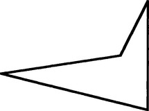
2. Two lino-cutter blades (trapeziums) are to be located from their corners. Consider images in which two corners of one blade are occluded by the other blade. Sketch the possible configurations, counting the number of corners in each case. If corners are treated like point features with no other attributes, show that the match graph will lead to an ambiguous solution. Show further that the ambiguity can in general be eliminated if proper account is taken of corner orientation. Specify how accurately corner orientation would need to be determined for this to be possible.

3. In Problem 15.2, would the situation be any better if the GHT were used?

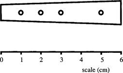
4. (a) Metal flanges are to be located from their holes using a graph matching (maximal clique) technique. Each bar has four identical holes at distances from the narrow end of the bar of 1, 2, 3, and 5 cm, as shown in Fig. 15.P1. Draw match graphs for the four different cases in which one ofthe four holes ofa given flange is obscured. In each case, determine whether the method is able to locate the metal flange without any error and whether any ambiguity arises.

Figure 15.P1

(b) Do your results tally with the results for human perception? How would any error or ambiguity be resolved in practical situations?

5. (a) Describe the maximal clique approach to object location. Explain why the largest maximal clique will normally represent the most likely solution to any object location task.

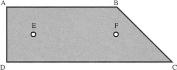
(b) If symmetrical objects with four feature points are to be located, show that suitable labeling of the object template will permit the task to be simplified. Does the type of symmetry matter? What happens in the case of a rectangle? What happens in the case of a parallelogram? (In the latter case, see points A, B, C, and D in Fig. 15.P2.)

Figure 15.P2

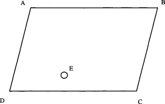
(c) A nearly symmetrical object with five feature points (see Fig. 15.P2) is to be located. This is to be achieved by looking initially for the feature points A, B, C, and D and ignoring the fifth point E. Discuss how the fifth point may be brought into play to finally determine the orientation of the object, using the maximal clique approach. What disadvantage might there be in adopting this two-stage approach?

6. (a) What is template matching? Explain why objects are normally located from their features rather than using whole object templates. What features are commonly used for this purpose?

(b) Describe templates that can be used for corner and hole detection.

(c) An improved type of lino-cutter blade (Fig. 15.P3) is to be placed into packs of six by a robot. Show how the robot vision system could locate the blades either from their corners or from their holes by applying the maximal clique method (i.e., show that both schemes would work).

Figure 15.P3

(d) After a time, it appears that the robot is occasionally confused when the blades overlap. It is then decided to locate the blades from their holes and their corners. Show why this helps to eliminate any confusion. Show also how finally distinguishing the corners from the holes can help in extreme cases of overlap.

7. (a) A certain type of lino-cutter blade has four corners and two fixing holes (Fig. 15.P4). Blades of this type are to be located using the maximal clique technique. Assume that the objects lie on a worktable and that they are viewed orthogonally at a known distance.

Figure 15.P4

(b) Draw match graphs for the following situations:

(i) the objects are to be located by their holes and their corners, regarding these as indistinguishable point features;

(ii) the objects are to be located solely by their corners (i.e., matching corners in the image with corners on an idealized object);

(iii) the objects are to be located solely by their holes;

(iv) the objects are to be located by their holes and their corners, but these are to be regarded as distinguishable features.

(c) Discuss your results with particular reference to:

(i) the robustness that can be achieved;

(ii) the speed of computation.

(d) In the latter case, distinguish the time taken to build the basic match graph from the time taken to find all the maximal cliques in it. State any assumptions you make about the time taken to find a maximal clique of m nodes in a match graph of n nodes.

8. (a) Decorative biscuits are to be inspected after first locating them from their holes. Show how the maximal clique graph matching technique can be applied to identify and locate the biscuits shown in Fig. 15.P5a, which are of the same size and shape.

Figure 15.P5

(b) Show how the analysis will be affected for biscuits that have an axis of symmetry, as shown in Fig. 15.P5b. Show also how the technique may be modified to simplify the computation for such a case.

(c) A more detailed model of the first type of biscuit shows it has holes of three sizes, as shown in Fig. 15.P5c. Analyze the situation and show that a much simplified match graph can be produced from the image data, leading to successful object location.

(d) A further matching strategy is devised to make use of the hole size information. Matches are only shown in the match graph if they arise between pairs of holes of different sizes. Determine how successful this strategy is, and discuss whether it is likely to be generally useful, for example, for objects with increased numbers of features.

(e) Work out an optimal object identification strategy, which will be capable of dealing with cases where holes and/or corners are to be used as point features, where the holes might have different sizes, where the corners might have different angles and orientations, where the object surfaces might have different colors or textures, and where the objects might have larger numbers of features. Make clear what the term optimal should be taken to mean in such cases.

9. (a) Figure 15.P6 shows a 2-D view of a widget with four corners. Explain how the maximal clique technique can be used to locate widgets even if they are partly obscured by various types of objects including other widgets.

Figure 15.P6 Diagram of a widget.

(b) Explain why the basic algorithm will not distinguish between widgets that are normally presented from those that are upside down. Consider how the basic method could be extended to ensure that a robot only picks up those that are the right way up.

(c) The camera used to view the widgets is accidentally jarred and then reset at a different, unknown height above the worktable. State clearly why the usual maximal clique technique will now be unable to identify the widgets. Discuss how the overall program could be modified to make sense of the data, and make correct interpretations in which all the widgets are identified. Assume first that widgets are the only objects appearing in the scene, and second that a variety of other objects may appear.

(d) The camera is jarred again, and this time is set at a small, unknown angle to the vertical. To be sure of detecting such situations and of correcting for them, a flat calibration object of known shape is to be stuck on the worktable. Decide on a suitable shape and explain how it should be used to make the necessary corrections.