
CHAPTER 19 Invariants and Their Applications
19.1 Introduction
Pattern recognition is a complex task and, as stated in Chapter 1, involves the twin processes of discrimination and generalization. Generalization is in many ways more important than discrimination—especially in the initial stages of recognition—since there is so much redundant information in a typical image. Thus, we need to find ways of helping to eliminate invalid matches. This is where the study of invariants comes into its own.
An invariant is a property of an object or class of objects that does not change with changes of viewpoint or object pose and that can therefore be used to help distinguish it from other objects. The procedure is to search for objects with a specific invariant, so that those that do not possess the invariant can immediately be discarded from consideration. An invariant property can be regarded as a necessary condition for an object to be in the chosen class, though in principle only detailed subsequent analysis will confirm that it is. In addition, if an object is found to possess the correct invariant, it will then be profitable to pursue the analysis further and find its pose, size, or other relevant data. Ideally, an invariant would uniquely identify an object as being of a particular type or class. Thus, an invariant should not merely be a property that leads to further hypotheses being made about the object, but one that fully characterizes it. However, the difference is a subtle one, more a matter of degree and purpose than an absolute criterion. We shall examine the extent of the difference by appealing to a number of specific cases.
Let us first consider an object being viewed from directly overhead at a known distance by a camera whose optical axis is normal to the plane on which the object is lying. We shall assume that the object is flat. Take two point features on the object such as corners or small holes (cf. Chapter 15). If we measure the image distance between these features, then this acts as an invariant, in that:
1. it has a value independent of the translation and orientation parameters of the object.
2. it will be unchanged for different objects of the same type.
3. it will in general be different from the distance parameters of other objects that might be on the object plane.
Thus measurement of distance provides a certain lookup or indexing quality that will ideally identify the object uniquely, though further analysis will be required to fully locate it and ascertain its orientation. Hence, distance has all the requirements of an invariant, though it could also be argued that it is only a feature that helps to classify objects. Here, we are ignoring an important factor—the effect of imprecision in measurement, owing to spatial quantization (or inadequate spatial resolution), noise, lens distortions, and so on. In addition, the effects of partial occlusion or breakage are also being ignored. Most definitely, there is a limit to what can be achieved with a single invariant measure, though in what follows we attempt to reveal what is possible, and we demonstrate the advantages of the way of thinking that involves analysis of invariants.
The above ideas relating to distance as an invariant measure showed it to be useful in suppressing the effects of translations and rotations of objects in 2-D. Hence, it is of little direct value when considering translations and rotations in 3-D. Furthermore, it is not even able to cope with scale variations of objects in 2-D. Moving the camera closer to the object plane and refocusing totally changes the situation: all values of the distance invariant residing in the object indexing table must be changed and the old values ignored. However, a moment’s thought will show that this last problem could be overcome. All we need to do is to take ratios of distances, which requires a minimum of three point features to be identified in the image and the interfeature distances measured. If we call two of these distances d1 and d2, then the ratio d1/d2 will act as a scale-independent invariant. That is, we will be able to identify objects using a single indexing operation whatever their 2-D translation, orientation, or apparent size or scale. An alternative to this idea is to measure the angle between pairs of distance vectors, cos-1 (d1.d2/|d1 ||d2|), which will again be scale invariant.
Of course, this consideration has already been invoked in our earlier work on shape analysis. If objects are subject only to 2-D translations and rotations but not to changes of scale, they can be characterized by their perimeters or areas as well as their normal linear dimensions. Furthermore, parameters such as compactness and aspect ratio, which employ dimensionless ratios of image measurements, were acknowledged in Chapter 6 to overcome the size/scale problem.
Nevertheless, the main motivation for using invariants is to obtain mathematical measures of configurations of object features, which are carefully designed to be independent of the viewpoint or coordinate system used and indeed do not require specific setup or calibration of the image acquisition system. However, it must be emphasized that camera distortions are assumed to be absent or to have been compensated for by suitable postcamera transformations (see Chapter 21).
19.2 Cross Ratios: The “Ratio of Ratios” Concept
It would be most useful if we could extend these ideas to permit indexing for general transformations in 3-D. An obvious question is whether finding ratios of ratios of distances will provide suitable invariants and lead to such a generalization. The answer is that ratios of ratios do provide useful further invariants, though going further than this leads to considerable complication, and there are restrictions on what can be achieved with limited computation. In addition, noise ultimately becomes a limiting factor, since so many parameters become involved in the computation of complex invariants that the method ultimately loses steam. (It becomes just one of many ways of raising hypotheses and therefore it has to compete with other approaches in a manner appropriate to the particular problem application being studied.)
We now consider the ratio of ratios approach. Initially, we only examine a set of four collinear points on an object. Figure 19.1 shows such a set of four points (P1, P2, P3, P4) and a transformation of them (Q1, Q2, Q3, Q4) such as that produced by an imaging system with optical center C (c, d). Choice of a suitable pair of oblique axes permits the coordinates of the points in the separate sets to be expressed respectively as:
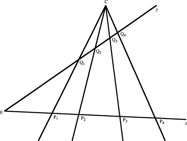
Figure 19.1 Perspective transformation of four collinear points. This figure shows four collinear points (P1, P2, P3, P4) and a transformation of them (Q1, Q2, Q3, Q4) similar to that produced by an imaging system with optical center C. Such a transformation is called a perspective transformation.
Taking points Pi, Qi, we can write the ratio CQi :PQi both as ![]() and as
and as ![]() . Hence:
. Hence:
which must be valid for all i. Subtraction of the i′th and j′th relations now gives:
Forming a ratio between two such relations will now eliminate the unknowns c and d. For example, we will have:
However, the result still contains factors such as X3/X2, which depend on absolute position. Hence, it is necessary to form a suitable ratio of such results, which cancels out the effects of absolute positions:
Thus, our original intuition that a ratio of ratios type of invariant might exist which would cancel out the effects of a perspective transformation is correct. In particular, four collinear points viewed from any perspective viewpoint yield the same value of the cross ratio, defined as above. The value of the cross ratio of the four points is written:
For clarity, we shall write this particular cross ratio as k in what follows. It should be noted that there are 4! = 24 possible ways in which 4 collinear points can be ordered on a straight line, and hence there could be 24 cross ratios. However, they are not all distinct; in fact, there are only six different values. To verify this, we start by interchanging pairs of points:
These cases provide the main possibilities, but of course interchanging more points will yield a limited number of further values—in particular:
This covers all six cases, and a moment’s thought (based on trying further interchanges of points) will show there can be no others. (We can only repeat k, 1—k, k/(k—1), and their inverses.) Of particular interest is the fact that numbering the points in reverse (which would correspond to viewing the line from the other side) leaves the cross ratio unchanged. Nevertheless, it is inconvenient that the same invariant has six different manifestations, for this implies that six different index values have to be looked up before the class of an object can be ascertained. On the other hand, if points are labeled in order along the line rather than randomly it should generally be possible to circumvent this situation.
So far we have been able to produce only one projective invariant, and this corresponds to the rather simple case of four collinear points. The usefulness of this measure is augmented considerably when it is noted that four collinear points, taken in conjunction with another point, define a pencil1 of concurrent coplanar lines passing through the latter point. It will be clear that we can assign a unique cross ratio to this pencil of lines, equal to the cross ratio of the collinear points on any line passing through them. We can clarify the situation by considering the angles between the various lines (Fig. 19.2). Applying the sine rule four times to determine the four distances in the cross ratio C(P1, P2, p3, p4) gives:
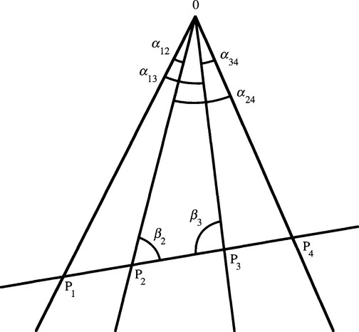
Figure 19.2 Geometry for calculation of the cross ratio of a pencil of lines. The figure shows the geometry required to calculate the cross ratio of a pencil of lines, in terms of the angles between them.
Substituting in the cross-ratio formula (equation (19.5)) and canceling the factors OP1, OP4, sin β2, and sin β3 now give:
Thus, the cross ratio depends only on the angles of the pencil of lines. It is interesting that appropriate juxtaposition of the sines of the angles gives the final formula invariance under perspective projection. Using the angles themselves would not give the desired degree of mathematical invariance. We can immediately see one reason for this: inversion of the direction of any line must leave the situation unchanged, so the formula must be tolerant to adding it to each of the two angles linking the line. This could not be achieved if the angles appeared without suitable trigonometric functions.
We can extend this concept to four concurrent planes, since the concurrent lines can be projected into four concurrent planes once a separate axis for the concurrency has been defined. Because there are infinitely many such axes, there are infinitely many ways in which sets of planes can be chosen. Thus, the original simple result on collinear points can be extended to a much more general case.
We started by trying to generalize the case of four collinear points, but what we achieved was first to find a dual situation in which points become lines also described by a cross ratio and then to find an extension in which planes are described by a cross ratio. We now return to the case of four collinear points, and we will see how we can extend it in other ways.
19.3 Invariants for Noncollinear Points
First, imagine that not all the points are collinear: specifically, let us assume that one point is not in the line of the other three. If this is the case, then there is not enough information to calculate a cross ratio. However, if a further coplanar point is available, we can draw an imaginary line between the noncollinear points to intersect their common line in a unique point, which will then permit a cross ratio to be computed (Fig. 19.3a.) Nevertheless, this is some way from a general solution to the characterization of a set of noncollinear points. We might inquire how many point features in general position2 on a plane will be required to calculate an invariant. The answer is five, since the fact that we can form a cross ratio from the angles between four lines immediately means that forming a pencil of four lines from five points defines a cross-ratio invariant (Fig. 19.3b).
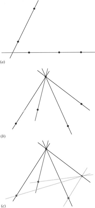
Figure 19.3 Calculation of invariants for a set of noncollinear points. (a) shows how the addition of a fifth point to a set of four points, one of which is not collinear with the rest, permits the cross ratio to be calculated. (b) shows how the calculation can be extended to any set of noncollinear points; also shown is an additional (gray) point which a single cross ratio fails to distinguish from other points on the same line. (c) shows how any failure to identify a point uniquely can be overcome by calculating the cross ratio of a second pencil generated from the five original points.
Although the value of this cross ratio provides a necessary condition for a match between two sets of five general coplanar points, it could be a fortuitous match, as the condition depends only on the relative directions between the various points and the reference point; that is, any of the nonreference points is only defined to the extent that it lies on a given line. Clearly, two cross ratios formed by taking two reference points will define the directions of all the remaining points uniquely (Fig. 19.3c).
We can now summarize the general result, which stipulates that for five general coplanar points, no three of which are collinear, two different cross ratios are required to characterize the shape. These cross ratios correspond to taking in turn two separate points and producing pencils of lines passing through them and (in each case) the remaining four points (Fig. 19.3c). Although it might appear that at least five cross ratios result from this sort of procedure, there are only two functionally independent cross ratios—essentially because the position of any point is defined once its direction relative to two other points is known.
Next, we consider the problem of finding the ground plane in practical situations—especially that of egomotion, including vehicle guidance (Fig. 19.4). Here a set of four collinear points can be observed from one frame to the next. If they are on a single plane, then the cross ratio will remain constant, but if one is elevated above the ground plane (as, for example, a bridge or another vehicle), then the cross ratio will vary over time. Taking a larger number of points, it should be possible to deduce by a process of elimination which are on the ground plane and which are not (though the amount of noise and clutter will determine the computational complexity of the task). All this is possible without any calibration of the camera, this being perhaps the main value of concentrating attention on projective invariants. Note that there is a potential problem regarding irrelevant planes, such as the vertical faces of buildings. The cross-ratio test is so resistant to viewpoint and pose that it merely ascertains whether the points being tested are coplanar. Only by using a sufficiently large number of independent sets of points can one plane be discriminated from another. (For simplicity we ignore any subsequent stages of pose analysis that might be carried out.)
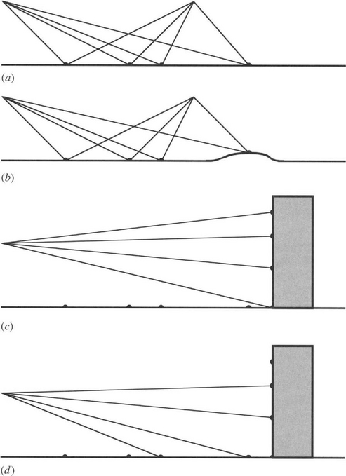
Figure 19.4 Use of cross ratio for egomotion guidance. (a) shows how the cross ratio for a set of four collinear points can be tracked to confirm that the points are collinear: this suggests that they lie on the ground plane. (b) shows a case where the cross ratio will not be constant. ) shows a case where all four points lie on planes, yet the cross ratio will not be constant.
19.3.1 Further Remarks about the 5-Point Configuration
The above description outlines the principles for solving the 5-point invariance problem but does not show the conditions under which it is guaranteed to operate properly. Actually, these are straightforward to demonstrate. First, the cross ratio can be expressed in terms of the sines of the angles α13, α24, α12, α34. Next, these can be reexpressed in terms of areas of relevant triangles, using equations typified by the following formula to express area:
Finally, the area can be reexpressed in terms of the point coordinates in the following way:
 (19.20)
Using this notation, a suitable final pair of cross ratio invariants for the configuration of five points may be written:
Although three more such equations may be written down, these will not be independent of the other two and will not carry any further useful information.
Note that a determinant will go to zero or infinity if the three points it relates to are collinear, corresponding to the situation when the area of the triangle is zero. When this happens any cross ratio containing this determinant will no longer be able to pass on any useful information. On the other hand, there is actually no further information to pass on, for this now constitutes a special case that is describable by a single cross ratio. We have reverted to the situation shown in Fig. 19.3a.
Finally, Fig. 19.3 misses one further interesting case: the situation of two points and two lines (Fig. 19.5). Constructing a line joining the two points and producing it until it meets the two lines, we then have four points on a single line. Thus, the configuration is characterized by a single cross ratio. Notice, too, that the two lines can be extended until they join, and further lines can be constructed from the join to meet the two points. This gives a pencil of lines characterized by a single cross ratio (Fig. 19.5c); the latter must have the same value as that computed for the four collinear points.
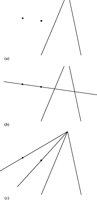
Figure 19.5 Cross ratio for two lines and two points. (a) Basic configuration. (b) How the line joining the two points introduces four collinear points to which a cross ratio may be applied. (c) How joining the two points to the junction of the two lines creates a pencil of four lines to which a cross ratio may be applied.
19.4 Invariants for Points on Conics
These discussions promote an understanding of how geometric invariants can be designed to cope with sets of points, lines, and planes in 3-D. Significantly more difficult is the case of curved lines and surfaces, though much headway has been made with regard to the understanding of conics and certain other surfaces (see Mundy and Zisserman, 1992a). It will not be possible to examine all such cases in depth here. However, it will be useful to consider conic sections, particularly ellipses, in more detail.
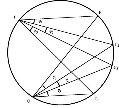
First, we consider Chasles’ (1855) theorem, which dates from the nineteenth century. (The history of projective geometry is quite rich and was initially carried out totally independently of the requirements of machine vision.) Suppose we have four fixed coplanar points F1, F2, F3, F4 on a conic section curve and one variable point P in the same plane (Fig. 19.6). Then the four lines joining P to the fixed points form a pencil whose cross ratio will in general vary with the position of P. Chasles’ theorem states that if P now moves so as to keep the cross ratio constant, then P will trace out a conic section. This provides a means of checking whether a set of points lies on a planar curve such as an ellipse. Note the close analogy with the problem of ground plane detection already mentioned. Again the amount of computation could become excessive if there were a lot of noise or clutter in the image. When the image contains N boundary features that need to be checked out, the problem complexity is intrinsically O(N5), since there are O(N4) ways of selecting the first four points, and for each such selection, N— 4 points must be examined to determine whether they lie on the same conic. However, choice of suitable heuristics would be expected to limit the computation. Note the problem of ensuring that the first four points are tested in the same order around the ellipse, which is liable to be tedious (1) for point features and (2) for disconnected boundary features.
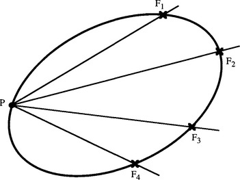
Figure 19.6 Definition of a conic using a cross ratio. Here P is constrained to move so that the cross ratio of the pencil from P to F1, F2, F3, F4 remains constant. By Chasles’ theorem, P traces out a conic curve.
Although Chasles’ theorem gives an excellent opportunity to use invariants to locate conics in images, it is not at all discriminatory. The theorem applies to a general conic, hence, it does not immediately permit circles, ellipses, parabolas, or hyperbolas to be distinguished, a fact that would sometimes be a distinct disadvantage. This is an example of a more general problem in pattern recognition system design—of deciding exactly how and in what sequence one object should be differentiated from another. Space does not permit this point to be considered further here.
Finally, we state without proof that all conic section curves can be transformed under perspective projection to other types of conic section, and thus into ellipses. Subsequently, they can be transformed into circles. Thus, any conic section curve can be transformed projectively into a circle, while the inverse transformation can transform it back again (Mundy and Zisserman, 1992b). This means that simple properties of the circle can frequently be generalized to ellipses or other conic sections. In this context, we should remember that, after perspective projection, lines intersecting curves do so in the same number of points, and thus tangents transform into tangents, chords into chords, three-point contact (in the case of nonconic curves) remains three-point contact, and so on. Returning to Chasles’ theorem, we see that a simple proof in the case of circles will automatically generalize to more complex conic section curves.
In response to this assertion, we can derive Chasles’ theorem almost trivially for a circle. Appealing to Fig. 19.7, we see that the angles Φ1, Φ2, Φ3 are equal to the respective angles y1, y2, y3 (angles in the same segment of a circle). Thus, the pencils PF1, PF2, PF3, PF4 and QF1, QF2, QF3, QF4 have equal angles, their relative directions being superposable. This means that they will have the same cross ratio, defined by equation (19.18). Hence, the cross ratio of the pencil will remain constant as P traces out the circle. As stated earlier, the property will automatically generalize to any other conic.
19.5 Differential and Semidifferential Invariants
Many attempts have been made to characterize continuous curves by invariants. The obvious way forward is to represent points on a curve in terms of local curve derivatives. If a sufficient number of these can be obtained, invariants can be formed and computed. However, the noise (including digitization noise) that always exists on curves limits the accuracy of higher derivatives, and as a result it is difficult to form useful invariants in this way. In general, the second derivative of the curve function is the highest that can normally be used, and this corresponds to curvature, which is only an invariant for Euclidean transformations (translation and rotation without change of scale).
As a result of this problem, semidifferential invariants are often used instead of differential invariants. They involve considering only a few “distinguished” points on curves and using these to generate invariants. The most common distinguished points to be used in this way are:
3. Cusps on curves (corners where the bounding tangents are coincident)
4. Bitangent points (points of contact of a line that touches the curve twice)
5. Other points whose locations can be derived from existing distinguished points by geometric constructions (see Fig. 19.8).
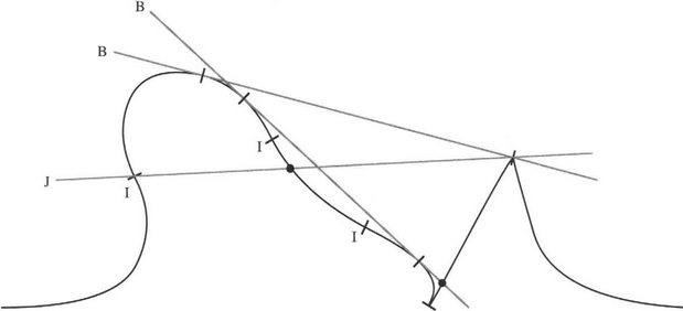
Figure 19.8 Means for finding distinguished points on a curve. The two bitangents contact the curve in a total of four bitangent points. Three points of inflection I provide another three distinguished points. A cusp and a corner provide a further two distinguished points (the latter also being a bitangent point). The line marked J contributes a further distinguished point on the curve, as does one of the bitangents: these are marked as large dots rather than as short lines.
Tangent points are unlikely to be suitable and so are not included in this list, as a smooth curve will have tangents along its entire length. This is because they are characterized merely by 2-point contact between a limiting chord and the curve. However, a point of inflection represents a 3-point contact, which means that it will be reasonably well localized, and its tangent will have a well-defined direction. On the other hand, bitangent points will be even more accurately represented, as the tangent direction will be accurately defined by two well-separated points on the curve (Fig. 19.8). Nevertheless, bitangent points will still incur some longitudinal error.
Bitangents can be of several sorts. In particular, they can contact the same shape on the same side; they can also cross the body and contact it on both sides. This latter case is more complex and is therefore sometimes discounted in machine vision applications. Nevertheless, it provides a means of finding further invariant reference points on an object. Note that this happens directly in that the bitangent points are already distinguished points. It also happens indirectly, as the bitangent may cross other reference lines—thereby defining further distinguished points. Figure 19.9 shows several cases of direct and indirect distinguished points, the most accurate of which arise from bitangents, while slightly less accurate ones arise from points of inflection.
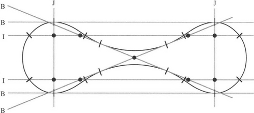
Figure 19.9 Means for finding direct and indirect distinguished points for an object. The four lines marked B are bitangents, which contribute six bitangent points. Two of the bitangents contact the object on opposite sides of its boundary. The two lines marked I arise from points of inflection. The two lines marked J are joins of bitangent points. The nine large dots are indirect distinguished points, which do not lie on the object boundary. Clearly, a good many more indirect distinguished points could be generated, though not all would have accurately defined locations.
Once enough distinguished points and reference lines between them have been found, cross ratio invariants may be obtained (1) from the incidence of distinguished points lying along suitable reference lines and (2) from pencils of lines drawn from distinguished points to line crossings or to other distinguished points.
A remark is needed to confirm that points of inflection can act as suitable distinguished points which are invariant under perspective transformations. Starting from the premise that perspective transformations preserve straight lines and points arising from crossings between curves and lines, we note that a chord that crosses a curve three times will also cross it three times under perspective projection. This will apply even when the three crossing points merge into 3-point contact.3 Hence, points of inflection are suitable distinguished points and are perspective-invariant.
This treatment has only dealt with planar curves and has not covered spatial nonplanar curves. The latter is a significantly more difficult area, as concepts such as bitangents and points of inflection have to be assigned new meaning in this more general domain. It is a subject we cannot broach here.
19.6 Symmetrical Cross Ratio Functions
When applying a cross ratio to a set of points on a line, the order of the points on the line is frequently known. This will almost certainly be the case if feature detection of an image is carried out in a forward raster scan. Hence, the only confusion in the ordering will be the direction in which the line has been traversed. However, the cross ratio is independent of the end from which the line is scanned, since C(P1, P2, P3, P4) = C(P4, P3, P2, P1). Nevertheless, in some situations the ordering of the cross ratio features will not be known with certainty. This may occur for the situations shown in Figs. 19.3 and 19.5, where the features themselves do not all lie on a single line; or where the features are angles; or where the points lie on a conic whose equation is as yet unknown. In such circumstances, it will be useful to have an invariant that takes in all possible orders of the features.
To derive such an invariant, note first that if there is a confusion in the ordering of the points such that the value could be either k or (1—k), then we could apply the function f(K) = k(1- k), which has the property f(K) = f(1—k), and this will solve the problem. Alternatively, if confusion exists between k and 1/k, then we can apply the function g(K) = k + 1/k, which has the property g(K) = g(1/K), and again this will solve the problem.
If there is potential confusion between the values k,(1—k) and 1/k, however, the situation becomes more complicated. It is difficult to write down any obvious function that satisfies the double condition h(K) = h(1—k) = h(1/K), though we may have soundly based intuition that it will involve symmetrical functions such as f(k) and g(K). The simplest answer seems to be:
which obeys the symmetry idea as it can be reexpressed in the two forms:
Fortunately, we need go no further in our quest to obey the six conditions required to recognize all six of the cross ratio values k,(1—k), 1/k, 1/(1—k), (k—1)/k, k/(k—1). The reason is that they are all deducible from each other by further applications of the initial negation and inversion rules. (The ultimate reason is that the operations to transform the function from one to another of the six forms form a group of order six, which is generated from the negation and inversion transforms.)
Although this is a powerful result, it does not come without loss. The reason is that a sixfold ambiguity is now inherent in the solution, so that once we have shown that the set of points satisfies the symmetrical cross ratio function, we still have to make tests to determine which of the six possibilities is the correct one. This is reflected by the complexity of the j-function, which contains a sixth degree polynomial and for every value of j there are six possible values of k (Fig. 19.10).
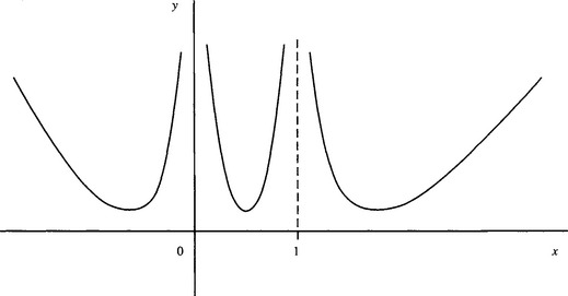
The situation can be described by stating that the function j(k) is not “complete,” in the sense that this function alone is insufficient to recognize the set of features unambiguously. To underline this fact, observe that the original cross ratio is complete. Once the value of k is known, we can uniquely determine the position of one of the points from the other three points. This is obvious from the graph of k as a function of x (where x = x34 gives the position of the fourth point4), which is a hyperbola:
19.7 Concluding Remarks
This chapter seeks to provide some insight into the important subject of invariants and its application in image recognition. The subject begins with consideration of ratios of ratios of distances, an idea that leads in a natural way to the cross ratio invariant. While its immediate manifestation lies in its application to recognition of the spacings of points on a line, it generalizes immediately to angular spacings for pencils of lines, as well as angular separations of concurrent planes. A further extension of the idea is the development of invariants that can describe sets of noncollinear points. It turns out that just two cross ratios suffice to characterize a set of four noncollinear points. The cross ratio can also be applied to conics. Indeed, Chasles’ theorem describes a conic as the locus of points that maintains a pencil of constant cross ratio with a given set of four points. However, this theorem does not permit one type of conic curve to be distinguished from another.
Many other theorems and types of invariant exist, but space prevents more than a mention of them here. As an extension to the line and conic examples given in this chapter, invariants have been produced which cover a conic and two coplanar nontangent lines, a conic and two coplanar points, and two coplanar conics. Of particular value is the group approach to the design of invariants (Mundy and Zisserman, 1992a). However, certain mathematically viable invariants, such as those that describe local shape parameters on curves, are too unstable for use in their full generality because of image noise. Nevertheless, semidifferential invariants have been shown (Section 19.5) to be capable of fulfilling essentially the same function.
Next, there is the warning of Åström (1995) that perspective transformations can produce such incredible changes in shape that a duck silhouette can be projected arbitrarily closely into something that looks like a rabbit or a circle, hence upsetting invariant-based recognition.5 Although such reports seem absent from the previous literature, Åström’s work indicates that care must be taken to regard recognition via invariants as hypothesis formation, which is capable of leading to false alarms.
Overall, the value of invariants lies in making computationally efficient checks of whether points or other features might form parts of specific objects. In addition, they make these checks without the necessity6 for camera calibration or knowledge of the camera’s viewpoint (though there is an implicit assumption that the camera is Euclidean). Although invariants have been known within the vision community for well over 30 years, only during the last 15 years have they been systematically developed and applied for machine vision. Such is their power that they will undoubtedly assume a stronger and more central role in the future. Indications of this role can be seen in Chapter 20 where they can help find vanishing points and in Chapter 24 where they are shown to be useful for the analysis of facial features.
Invariants are central to pattern recognition—reflecting within-class constancy vis-à-vis between-class variance. This chapter has shown that in 3-D vision, they are especially valuable in providing a hedge against the problems of perspective projection. Perhaps oddly, the cross ratio invariant always seems to emerge, in one guise or another, in 3-D vision.
19.8 Bibliographical and Historical Notes
The mathematical subject of invariance is very old (cf. the work of Chasles, 1855), but only recently has it been developed systematically for machine vision. Notable in this context is the work of Rothwell, Zisserman, and their co-workers, as reported by Forsyth et al. (1991), Mundy and Zisserman (1992a,b), Rothwell, et al. (1992a,b), and Zisserman et al., (1990). In particular, the paper by Forsyth et al. (1991) both shows the range of available invariant techniques and discusses problems of stability that arise in certain cases. The appendix (Mundy and Zisserman, 1992b) on projective geometry for machine vision, which appears in Mundy and Zisserman (1992a), is especially valuable and provides the background needed for understanding the other papers in the volume. This volume has a theoretical flavor that demonstrates what ought to be possible using invariants, though comparisons between invariants and other approaches to recognition are perhaps lacking. Thus, only by examining whether workers choose to use invariants in real applications will the full story emerge. In this respect, the paper by Kamel et al. (1994) on face recognition is of great interest, for it shows how invariants helped to achieve more than had been achieved earlier after many attempts using other approaches—specifically in correcting for perspective distortions during face recognition.
Other more recent work appears in a Special Issue of Image and Vision Computing (Mohr and Wu, 1998). In particular, the paper by Van Gool et al. (1998) shows how shadows can be allowed for in aerial images, and the paper by Boufama et al. (1998) shows how invariants can help with object positioning. Startchik et al. (1998) provides a useful demonstration of the semidifferential invariant methods covered in Section 19.5. Maybank (1996) deals with the problem of accuracy with invariants, making the point that this can be serious even for cross ratios (which contain only four parameters). Another early work, by a totally different set of workers, is Barrett et al. (1991) and contains a number of useful derivations, together with a practical example of aircraft recognition, complete with accuracy assessments.
Rothwell’s (1995) book covers the early work on invariance in a thoughtful manner, and the later 3-D books by Hartley and Zisserman (2000) and Faugeras and Luong (2001) integrate the ideas into their structure but are not always easy to understand by students starting out in the subject. Semple and Kneebone (1952) is a standard work on projective geometry, which is still widely used in one or another reprint.
19.9 Problems
1. Find a symmetrical cross ratio function p(k) that has the same value for all cyclic permutations of the four points A, B, C, D on a straight line. Show also that p(k) is incomplete but that it has just two values for each position of point D on the line.
2. Show that the six operations required to transform the cross ratio k into the six different values for four points on a line form a group G of order six (see Sections 19.2 and 19.6). Show that G is a noncyclic group and has two subgroups of order 2 and 3, respectively. Hint: Show that all possible combined operations fall within the same set of six and that this set contains the identity operation and the inverses of all the elements of the set.
3. Show that a conic and two points can be used to define an invariant cross ratio.
4. Show that two conics can be used to define an invariant cross ratio (a) if they intersect in four points, (b) if they intersect in two points, (c) if they do not intersect at all, as long as they have common tangents.7
5. (a) Perform a geometric calculation based on the sine rule which shows that the angles a, //, y are related to the distances a, b, c in Fig. 19.P1 by the equation:
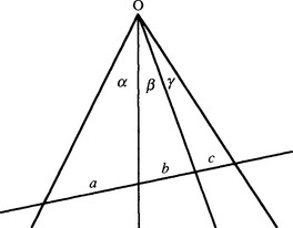
(b) Show that this equation leads to a relation between the cross ratios for various distances on the line and for the sines of various angles. Hence, show that this also leads to the constancy of the cross ratios on any two lines crossing the pencil of four lines passing though O.
6. (a) Explain the value of using invariants in relation to pattern recognition systems. Illustrate your answer by considering the value of thinning algorithms in optical character recognition.
(b) The cross ratio of four points (P1, P2, P3, P4) on a line is defined as the ratio:
Explain why this is a useful type of invariant for objects viewed under full perspective projection. Show that labeling the points in reverse order will not change the value of the cross ratio.
(c) Give arguments why the cross ratio concept should also be valid for weak perspective projection. Work out a simpler invariant that is valid for straight lines viewed under weak perspective projection.
(d) A flat lino-cutter blade has two parallel sides of different lengths: it is viewed under weak perspective projection. Discuss whether it can be identified from any orientation in 3-D by measuring the lengths of its sides.
7. (a) Flagstones are viewed on a pavement, providing a large number of coplanar feature points. Show that a correspondence can be made between five coplanar feature points in two images—however the camera has been moved between the shots—by checking the values of two cross ratios.
(b) It is required that a panorama of a scene be composed by taking a number of photographs and “stitching” them together after making appropriate image transformations. For this purpose, it is necessary to make correspondences between the images. Show that the two cross ratio types of planar invariants can be used for this purpose, even if the chosen scene features do not lie on a common plane. Determine under what conditions this is possible.
1 It is a common nomenclature of projective geometry to call a set of concurrent lines a pencil (e.g., Tuckey and Armistead, 1953).
2 Points on a plane are described as being in general position if they are chosen at random and are not collinear or in any special pattern such as a regular polygon.
3 Three-point contact is distinguishable from 2-point contact in that the tangent crosses the curve at the point of contact.
4 In projective geometry it is well known that there are three degrees of freedom on a line: the positions of three points on a line are not predictable from other views of the three points, without further information on the viewpoint.
5 It could, of course, be argued that all recognition methods will be subject to the effects of perspective transformations. However, invariant-based recognition will not flinch from invoking highly extreme transformations that appear to grossly distort the objects in question, whereas more conventional methods are likely to be designed to cope with a reasonable range of expected shape distortions.
6 Here we assume that the aim is location of specific objects in the image. If the objects are then to be located in the world coordinates, camera calibration or some use of reference points will of course be needed. However, there are many applications, such as inspection, surveillance, and identification (e.g., of faces or signatures) where location of objects in the image can be entirely adequate.
7 The case of nonintersecting conics with no common tangents requires complex algebra: see, for example, Rothwell (1995). The possibility of ambiguity and incompleteness in cases (a)-(c) is also discussed in Rothwell (1995).