
CHAPTER 22 Automated Visual Inspection
22.1 Introduction
Over the past two decades, machine vision has consolidated its early promise and has become a vital component in the design of advanced manufacturing systems. On the one hand, it provides a means of maintaining control of quality during manufacture, and on the other, it is able to feed the assembly robot with the right sort of information to construct complex products from sets of basic components. Automated assembly helps to make flexible manufacture a reality, so that costs due to underuse of expensive production lines are virtually eliminated.
These two major applications of vision—automated visual inspection and automated assembly—have many commonalities and can on the whole be performed by similar hardware vision systems employing closely related algorithms. Perhaps the most obvious use of visual inspection is to check products for quality so that defective ones may be rejected. This is easy to visualize in the case of a line making biscuits or washers at rates of the order of one million per day. Another area of application of inspection is to measure a specific parameter for each product and to feed its value back to an earlier stage in the plant in order to “close the loop” of the manufacturing process. A typical application is to adjust the temperature of jam or chocolate in a biscuit factory when the coating is found not to be spreading correctly. A third use of inspection is simply to gather statistics on the efficiency of the manufacturing process, finding, for example, how product diameters vary, in order to provide information that will help management with advance planning.
Another aspect of inspection is what can be learned via other modalities such as X-rays, even if the acquired images often ressemble visible light images. Similarly, it is relevant to ask what additional information color can provide that is useful for inspection. Sections 22.10 and 22.11 aim to give answers to these questions.
In automated assembly, vision can provide feedback to control the robot arm and wrist. For this purpose it needs to provide detailed information on the positions and orientations of objects within the field of view. It also needs to be able to distinguish individual components within the field of view. In addition, a well-designed vision system will be able to check components before assembly, for example, so as to prevent the robot from trying to fit a screw into a nonexistent hole.
Inspection and assembly require virtually identical vision systems, the most notable difference often being that a linescan camera is used for inspecting components on a conveyor, whereas an area (whole picture) camera is required for assembly operations on a worktable. The following discussion centers on inspection, although, because of the similarity of the two types of application, many of the concepts that are developed are also useful for automated assembly tasks.
22.2 The Process of Inspection
Inspection is the process of comparing individual manufactured items against some preestablished standard with a view to maintenance of quality. Before proceeding to study inspection tasks in detail, it is useful to note that the process of inspection commonly takes place in three definable stages:
We defer detailed discussion of image acquisition until Chapter 27 and comment here on the relevance of separating the processes of location and scrutiny. This is important because (either on a worktable or on a conveyor) large numbers of pixels usually have to be examined before a particular product is found, whereas once it has been located, its image frequently contains relatively few pixels, and so rather little computational effort need be expended in scrutinizing and measuring it. For example, on a biscuit line, products may be separated by several times the product diameter in two dimensions, so that some 100,000 pixels may need to be examined to locate products occupying say 5000 pixels. Product location is therefore likely to be a much more computationally intensive problem than product scrutiny. Although this is generally true, sampling techniques may permit object location to be performed with much increased efficiency (Chapter 10). Under these circumstances, location may be faster than scrutiny, since the latter process, though straightforward, tends to permit no shortcuts and requires all pixels to be examined.
22.3 Review of the Types of Objects to Be Inspected
Before studying methods of visual inspection (including those required for assembly applications), we should consider the types of objects with which such systems may have to cope. As an example, we can take two rather opposing categories: (1) goods such as food products that are subject to wide variation during manufacture but for which physical appearance is an important factor, and (2) those products such as precision metal parts which are needed in the electronics and automotive industries. The problems specific to each category are discussed first; then size measurement and the problem of 3-D inspection are considered briefly.
22.3.1 Food Products
Food products are a particularly wide category, ranging from chocolate cream biscuits to pizzas, and from frozen food packs to complete set meals (as provided by airlines). In the food industry, the trend is toward products of high added value. Logically, such products should be inspected at every stage of manufacture, so that further value is not added to products that are already deficient. However, inspection systems are still quite expensive, and the tendency is to inspect only at the end of the product line. This procedure at least ensures (1) that the final appearance is acceptable and (2) that the size of the product is within the range required by the packaging machine.1 This strategy is reasonable for many products—as for some types of biscuit where a layer of jam is clearly discernible underneath a layer of chocolate. Pizzas exemplify another category wherein many additives appear on top of the final product, all of which are in principle detectable by a vision system at the end of the product line.
When checking the shapes of chocolate products (chocolates, chocolate bars, chocolate biscuits, etc.), a particular complication that arises is the “footing” around the base of the product. This footing is often quite jagged and makes it difficult to recognize the product or to determine its orientation. However, the eye generally has little difficulty with this task, and hence if a robot is to place a chocolate in its proper place in a box it will have to emulate the eye and employ a full gray-scale image; shortcuts with silhouettes in binary images are unlikely to work well. In this context, it should be observed that chocolate is one of the more expensive ingredients of biscuits and cakes. A frequently recurring inspection problem is to check that chocolate cover is sufficient to please the consumer while low enough to maintain adequate profit margins.
Returning to packaged meals, we find that these present both an inspection and an assembly problem. A robot or other mechanism has to place individual items on the plastic tray, and it is clearly preferable that every item should be checked to ensure, for example, that each salad contains an olive or that each cake has the requisite blob of cream.
22.3.2 Precision Components
Many other parts of industry have also progressed to the automatic manufacture and assembly of complex products. It is necessary for items such as washers and O-rings to be tested for size and roundness, for screws to be checked for the presence of a thread, and for mains plugs to be examined for the appropriate pins, fuses, and screws. Engines and brake assemblies also have to be checked for numerous possible faults. Perhaps the worst problems arise when items such as flanges or slots are missing, so that further components cannot be fitted properly. It cannot be emphasized enough that what is missing is at least as important as what is present. Missing holes and threads can effectively prevent proper assembly. It is sometimes stated that checking the pitch of a screw thread is unnecessary—if a thread is present, it is bound to be correct. However, there are many industrial applications where this is not true.
Table 22.1 summarizes some of the common features that need to be checked when dealing with individual precision components. Note that measurement of the extent of any defect, together with knowledge of its inherent seriousness, should permit components to be graded according to quality, thereby saving money for the manufacturer. (Rejecting all defective items is a very crude option.)
22.3.3 Differing Requirements for Size Measurement
Size measurement is important both in the food industry and in the automotive and small-parts industry. However, the problems in the two cases are often rather different. For example, the diameter of a biscuit can vary within quite wide limits (∼5%) without giving rise to undue problems, but when it gets outside this range there is a serious risk of jamming the packing machine, and the situation must be monitored carefully. In contrast, for mechanical parts, the required precision can vary from 1% for objects such as O-rings to 0.01% for piston heads. This variation makes it difficult to design a truly general-purpose inspection system. However, the manufacturing process often permits little variation in size from one item to the next. Hence, it may be adequate to have a system that is capable of measuring to an accuracy of rather better than 1%, as long as it is capable of checking all the characteristics mentioned in Table 22.1.
Table 22.1 Features to be checked on precision components
| Dimensions within specified tolerances |
| Correct positioning, orientation, and aUgnment |
| Correct shape, especially roundness, of objects and holes |
| Whether corners are misshapen, blunted, or chipped |
| Presence of holes, slots, screws, rivets, and so on |
| Presence of a thread on screws |
| Presence of burr and swarf |
| Pits, scratches, cracks, wear, and other surface marks |
| Quality of surface finish and texture |
| Continuity of seams, folds, laps, and other joins |
When high precision is vital, accuracy of measurement should be proportional to the resolution of the input image. Currently, images of up to 512 × 512 pixels are common, so accuracy of measurement is basically of the order of 0.2%. Fortunately, gray-scale images provide a means of obtaining significantly greater accuracy than indicated by the above arguments, since the exact transition from dark to light at the boundary of an object can be estimated more closely. In addition, averaging techniques (e.g., along the side of a rectangular block of metal) permit accuracies to be increased even further—by a factor ![]() if N pixel measurements are made. These factors permit measurements to be made to subpixel resolution, sometimes even down to 0.1 pixel.
if N pixel measurements are made. These factors permit measurements to be made to subpixel resolution, sometimes even down to 0.1 pixel.
22.3.4 Three-dimensional Objects
All real objects are 3-D, although the cost of setting up an inspection station frequently demands that they be examined from one viewpoint in a single 2-D image. This requirement is highly restrictive and in many cases overrestrictive. Nevertheless, generally an enormous amount of useful checking and measurement can be done from one such image. The clue that this is possible lies in the prodigious capability of the human eye—for example, to detect at a glance from the play of light on a surface whether or not it is flat. Furthermore, in many cases products are essentially flat, and the information that we are trying to find out about them is simply expressible via their shape or via the presence of some other feature that is detectable in a 2-D image. In cases where 3-D information is required, methods exist for obtaining it from one or more images, for example, via binocular vision or structured lighting, as has already been seen in Chapter 16. More is said about this in the following sections.
22.3.5 Other Products and Materials for Inspection
This subsection briefly mentions a few types of products and materials that are not fully covered in the foregoing discussion. First, electronic components are increasingly having to be inspected during manufacture, and, of these, printed circuit boards (PCBs) and integrated circuits are subject to their own special problems, which are currently receiving considerable attention. Second, steel strip and wood inspection are also very important. Third, bottle and glass inspection has its own particular intricacies because of the nature of the material. Glints are a relevant factor—as it also is in the case of inspection of cellophane-covered foodpacks. In this chapter, space permits only a short discussion of some of these topics (see Sections 22.7 and 22.8).
22.4 Summary—The Main Categories of Inspection
The preceding sections have given a general review of the problems of inspection but have not shown how they might be solved. This section takes the analysis a stage further. First, note that the items in Table 22.1 may be classified as geometrical (measurement of size and shape—in 2-D or 3-D as necessary), structural (whether there are any missing items or foreign objects), and superficial (whether the surface has adequate quality). As is evident from Table 22.1, these three categories are not completely distinct, but they are useful for the following discussion.
Start by noting that the methods of object location are also inherently capable of providing geometrical measurements. Distances between relevant edges, holes, and corners can be measured; shapes of boundaries can be checked both absolutely and via their salient features; and alignments can usually be checked quite simply, for example, by finding how closely various straight-line segments fit to the sides of a suitably placed rectangle. In addition, shapes of 3-D surfaces can be mapped out by binocular vision, photometric stereo, structured lighting, or other means (see Chapter 16) and subsequently checked for accuracy.
Structural tests can also be made once objects have been located, assuming that a database of the features they are supposed to possess is available. In the latter case, it is necessary merely to check whether the features are present in predicted positions. As for foreign objects, these can be looked for via unconstrained search as objects in their own right. Alternatively, they may be found as differences between objects and their idealized forms, as predicted from templates or other data in the database. In either case, the problem is very data-dependent, and an optimal solution needs to be found for each situation. For example, scratches may be searched for directly as straight-line segments.
Tests of surface quality are perhaps more complex. Chapter 27 describes methods of lighting that illuminate flat surfaces uniformly, so that variations in brightness may be attributed to surface blemishes. For curved surfaces, it might be hoped that the illumination on the surface would be predictable, and then differences would again indicate surface blemishes. In complex cases, however, probably the only alternative is to resort to the use of switched lights coupled with rigorous photometric stereo techniques (see Chapter 16). Finally, it should be noted that the problem of checking quality of surface finish is akin to that of ensuring an attractive physical appearance, and this judgment can be highly subjective. Inspection algorithms therefore need to be “trained” in some way to make the right judgments. (Note that judgments are decisions or classifications, and so the methods of Chapter 24 are appropriate.)
Accurate object location is a prerequisite to reliable object scrutiny and measurement, for all three main categories of inspection. If a CAD system is available, then providing location information permits an image to be generated which should closely match the observed image. Template matching (or correlation) techniques should in many cases permit the remaining inspection functions to be fulfilled. However, this will not always work without trouble, as when object surfaces have a random or textured component. Preliminary analysis of the texture may therefore have to be carried out before relevant templates can be applied—or at least checks made of the maximum and minimum pixel intensities within the product area. More generally, in order to solve this and other problems, some latitude in the degree of fit should be permitted.
The same general technique—that of template matching—arises in the measurement and scrutiny phase as in the object location phase. However (as remarked earlier), this need not consume as much computational effort as in object location. The underlying reason is that template matching is difficult when there are many degrees of freedom inherent in the situation, since comparisons with an enormous number of templates may be required. However, when the template is in a standard position relative to the product and when it has been oriented correctly, template matching is much more likely to constitute a practical solution to the inspection task, although the problem is very data-dependent.
Despite these considerations, it is necessary to find a computationally efficient means of performing the checks of parts. The first possibility is to use suitable algorithms to model the image intensity and then to employ the model to check relevant surfaces for flaws and blemishes. Another useful approach is to convert 2-D to 1-D intensity profiles. This approach leads to the lateral histogram (Chapter 13) and radial histogram techniques. The histogram technique can conveniently be applied for inspecting the very many objects possessing circular symmetry, as will be seen later. First we consider a simple but useful means of checking shapes.
22.5 Shape Deviations Relative to a Standard Template
For food and certain other products, an important factor in 2-D shape measurement is the deviation relative to a standard template. Maximum deviations are important because of the need to fit the product into a standard pack. Another useful measure is the area of overflow or underfill relative to the template (Fig. 22.1). For simple shapes that are bounded by circular arcs or straight lines (a category that includes many types of biscuits or brackets), it is straightforward to test whether a particular pixel on or near the boundary is inside the template or outside it. For straight-line segments this is achieved in the following way. Taking the pixel as (x1, y1) and the line as having equation:
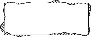
Figure 22.1 Measurement of product area relative to a template. In this example, two measurements are taken, indicating, respectively, the areas of overflow and underfill relative to a prespecified rectangular template.
the coordinates of the pixel are substituted in the expression:
The sign will be positive if the pixel lies on one side of the line, negative on the other, and zero if it is on the idealized boundary. Furthermore, the distance on either side of the line is given by the formula:
The same observation about the signs applies to any conic curve if appropriate equations are used. For example, for an ellipse:
where f(x, y) changes sign on the ellipse boundary. For a circle the situation is particularly simple, since the distance to the circle center need only be calculated and compared with the idealized radius value. For more complex shapes, deviations need to be measured using centroidal profiles or the other methods described in Chapter 7. However, the method we have outlined is useful, for it is simple, quick, and reasonably robust, and does not need to employ sequential boundary tracking algorithms; a raster scan over the region of the product is sufficient for the purpose.
22.6 Inspection of Circular Products
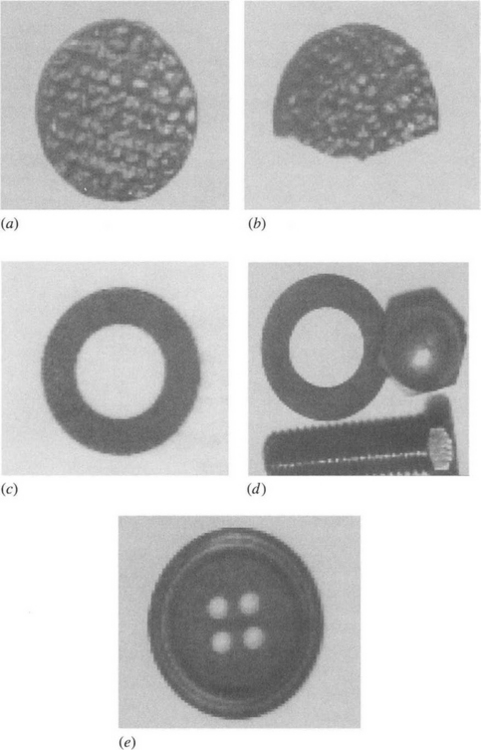
Since circular products are so common, it has proved beneficial to develop special techniques for scrutinizing them efficiently. The “radial histogram” technique was developed for this purpose (Davies, 1984c, 1985b). It involves plotting a histogram of intensity as a function of radial distance from the center. Varying numbers of pixels at different radial distances complicate the problem, but smooth histograms result when suitable normalization procedures are applied (Figs. 22.2 and 22.3). These give accurate information on all three major categories of inspection. In particular, they provide values of all relevant radii. For example, both radii of a washer can be estimated accurately using this technique. Surprisingly, accuracy can be as high as 0.3% even when objects have radii as low as 40 pixels (Davies, 1985c), with correspondingly higher accuracies at higher resolutions.
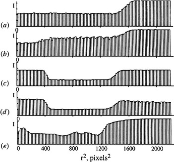
Figure 22.2 Practical applications of the radial histogram approach. In all cases, an r2 base variable is used, and histogram columns are individually normalized. This corresponds to method (iv) in the text (Section 22.6.1). These histograms were generated from the original images of Fig. 22.3.
Radial histograms are particularly well suited to the scrutiny of symmetrical products that do not exhibit a texture, or for which texture is not prominent and may validly be averaged out. In addition, the radial histogram approach ignores correlations between pixels in the dimension being averaged (i.e., angle). Where such correlations are significant it is not possible to use the approach. An obvious example is in the inspection of components such as buttons, where angular displacement of one of four button holes will not be detectable unless the hole encroaches on the space of a neighboring hole. Similarly, the method does not permit checking the detailed shape of each small hole. The averaging involved in finding the radial histogram mitigates against such detailed inspection, which is then best carried out by separate direct scrutiny of each of the holes.
22.6.1 Computation of the Radial Histogram: Statistical Problems
In computing the radial intensity histogram of a region in an image, one of the main variables to be considered is the radial step size s. If s is small, then few pixels contribute to the corresponding column of the histogram, and little averaging of noise and related effects takes place. For textured products, this could be a disadvantage unless it is specifically required to analyze texture by an extension of the method. Ignoring the latter possibility and increasing s in order to obtain a histogram having a statistically significant set of ordinates are bound to result in a loss in radial resolution. To find more about this tradeoff between radial resolution and accuracy, it is necessary to analyze the statistics of interpixel (radial) distances. Assuming a Poisson distribution for the number of pixels falling within a band of a given radius and variable s, we find that histogram column height or “signal” varies, at the given radius, as the step size s, whereas “noise” varies as![]() giving an overall signal-to-noise ratio varying (for the given radius) as
giving an overall signal-to-noise ratio varying (for the given radius) as ![]() . Radial resolution is, of course, inversely proportional to s. For small radii, those of less than about 20 pixels, this simple model is inaccurate, and it is better to follow the actual detailed statistics of a discrete square lattice. Under these circumstances, it seems prudent to examine the pixel statistics plotted in Fig. 22.4 for various values of s and from these to select a value of s which is the best compromise for the application being considered.
. Radial resolution is, of course, inversely proportional to s. For small radii, those of less than about 20 pixels, this simple model is inaccurate, and it is better to follow the actual detailed statistics of a discrete square lattice. Under these circumstances, it seems prudent to examine the pixel statistics plotted in Fig. 22.4 for various values of s and from these to select a value of s which is the best compromise for the application being considered.
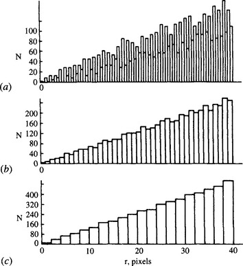
Figure 22.4 Pixel statistics for various radial step sizes; the number of pixels, as a function of radius, that fall into bands of given radial step size. The chosen step sizes are (a) 0.50, (b) 1.00, and (c) 2.00 pixels.
For many applications, it is inconvenient to have radial intensity distributions such as that depicted in Fig. 22.5, in which the column height varies inherently as the radius because the number of pixels in a band of radius r and given s is (approximately) proportional to r. It is more convenient to normalize the distribution so that regions of uniform intensity give rise to a uniform radial intensity distribution. This uniformity may be achieved in two ways. The first is to multiply each column of the radial histogram by a factor that brings it to an inherently uniform value. The other is to plot the histogram as a function of some function u(r) other than r which gives the same effect.
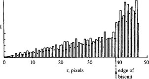
Figure 22.5 Basic form of radial intensity distribution, which varies approximately as the radius. The product being inspected here is the biscuit of Fig. 22.3a.
Taking the latter approach first, we find that changing variables from r to u(r) results in
 (22.5)
We now require that I(u) = constant for fixed step size δu. Setting δu equal to a constant leads to
as might indeed have been expected. In addition, note that
making the histogram base parameter equal to r2 (within a constant of proportionality).
Unfortunately, this approach is still affected by the pixel statistics problem, as shown in Fig. 22.6. Thus, we are effectively being forced to apply the approach of normalizing the histogram by multiplying by suitable numerical factors, as suggested earlier. There are now four alternatives:
1. Use the basic radial histogram.
2. Use the modified radial histogram, with u(r) = r2 base parameter.
3. Use the basic histogram, with individual column normalization.
4. Use the u(r) = r2 histogram, with individual column normalization.
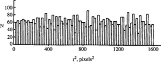
Figure 22.6 Pixel statistics for an r2 histogram base parameter. The pixel statistics are not exactly uniform even when the radial histogram is plotted with an r2 base parameter.
As a rule, it appears to be necessary to normalize each column of the histogram individually to obtain the most accurate results. For ease of interpretation, it would also be preferable to use the modified base parameter u(r) = r2 rather than r.
Note that the square-law approach is trivial to implement, since r2 rather than r is the value that is actually available during computation (r has to be derived from r2 if it is needed). Furthermore, the r2 base parameter gives a nonlinear stretch to the histogram which matches the increased radial accuracy that is actually available at high values of r. This means that the u(r) = r2 histogram permits greater accuracy in the estimation of radius at large r than it does at small r, thus making u(r) = r2 the natural base variable to employ (Davies, 1985b).
These considerations make method (4) the most generally suitable one, although method (2) is useful when speed of processing is a particular problem. Finally, it is relevant to note that, to a first approximation, all types of radial intensity histograms mentioned earlier can eliminate the effects of a uniform gradient of background illumination over an object.
22.6.2 Application of Radial Histograms
Figure 22.2 shows practical applications of the above theory to various situations, depicted in Fig. 22.3: see also Fig. 22.7, which relates to the biscuits shown in Fig. 10.1. In particular, notice that the radial histogram approach is able to give vital information on various types of defects: the presence or absence of holes in a product such as a washer or a button, whether circular objects are in contact or overlapping, broken objects, “show-through” of the biscuits where there are gaps in a chocolate or other coating, and so on. In addition, it is straightforward to derive dimensional measurements from radial histograms. In particular, radii of discs or washers can be obtained to significantly better than 1 pixel accuracy because of the averaging effect of the histogram approach. However, the method is limited here by the accuracy with which the center of the circular region is first located. This underlines the value of the high-accuracy center finding technique of Chapter 10. To a certain extent, accuracy is limited by the degree of roundness of the product feature being examined. Radius can be measured only to the extent that it is meaningful! In this context, it is worth emphasizing that the combination of techniques described here is not only accurate but also sparing in computation.
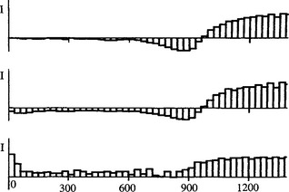
Figure 22.7 Radial intensity histograms for the three biscuits of Fig. 10.1. The order is from top to bottom in both figures. Intensity here is measured relative to that at the center of an ideal product.
It might be imagined that the radial histogram technique is applicable only for symmetrical objects. However, it is also possible to use radial histograms as signatures of intensity patterns in the region of specific salient features. Small holes are suitable salient features, but corners are less suitable unless the background is saturated out at a constant value. Otherwise, too much variation arises from the background, and the technique does not prove viable.
Finally, note that the radial histogram approach has the useful characteristic that it is trainable, since the relevant 1-D templates may be accumulated, averaged over a number of ideal products, and stored in memory, ready for comparisons with less ideal products. This characteristic is valuable, not only because it provides convenience in setting up but also because it permits inspection to be adaptable to cover a range of products.
22.7 Inspection of Printed Circuits
Over the past two or three decades, machine vision has been used increasingly in the electronics industry, notably for inspecting printed circuit boards (PCBs). First, PCBs may be inspected before components are inserted; second, they may be inspected to check that the correct components have been inserted the correct way round; and third, all the soldered joints may be scrutinized. The faults that have to be checked for on the boards include touching tracks, whisker bridges, broken tracks (including hairline cracks), and mismatch between pad positions and holes drilled for component insertion. Controlled illumination is required to eliminate glints from the bare metal and to ensure adequate contrast between the metal and its substrate. With adequate control over the lighting, most of the checks (e.g., apart from reading any print on the substrate) may be carried out on a binarized image, and the problem devolves into that of checking shape. The checking may be tackled by gross template matching—using a logical exclusive-or operation—but this approach requires large data storage and precise registration has to be achieved.
Difficulties with registration errors can largely be avoided if shape analysis is performed by connectedness measurement (using thinning techniques) and morphological processing. For example, if a track disappears or becomes broken after too few erosion operations, then it is too narrow. A similar procedure will check whether tracks are too close together. Similarly, hairline cracks may be detected by dilations followed by tests to check for changes in connectedness.
Alignment of solder pads with component holes is customarily checked by employing a combination of back and front lighting. Powerful back lighting (i.e., from behind the PCB) gives bright spots at the hole positions, while front lighting gives sufficient contrast to show the pad positions. It is then necessary to confirm that each hole is, within a suitable tolerance, at the center of its pad. Counting of the bright spots from the holes, plus suitable measurements around hole positions (e.g., via radial histogram signatures), permits this process to be performed satisfactorily.
The main problem with PCB inspection is the resolution required. Typically, images have to be digitized to at least 4000 × 4000 pixels—as when a 20 × 20 cm board is being checked to an accuracy of 50 μm. In addition, a suitable inspection system normally has to be able to check each board fully in less than one minute. It also has to be trainable, to allow for upgrades in the design of the circuit or improvements in the layout. Finally, it should cost no more than $60,000. However, considerable success has been attained with these aims.
To date, the bulk of the work in PCB inspection has concerned the checking of tracks. Nevertheless, useful work has also been carried out on the checking of soldered joints. Here, each joint has to be modeled in 3-D by structured light or other techniques. In one such case, light stripes were used (Nakagawa, 1982), and in another, surface reflectance was measured with a fixed lighting scheme (Besl et al., 1985). Note that surface brightness says something about the quality of the soldered joint. This type of problem is probably completely solvable (at least up to the subjective level of a human inspector), but detailed scrutiny of each joint at a resolution of say 64 × 64 pixels may well be required to guarantee that the process is successful. This implies an enormous amount of computation to cope with the several hundreds (or in some cases thousands) of joints on most PCBs. Hence, special architectures were needed to handle the information in the time available.
Similar work is under way on the inspection of integrated circuit masks and die bonds, but space does not permit discussion of this rapidly developing area. For a useful review, see Newman and Jain (1995).
22.8 Steel Strip and Wood Inspection
The problem of inspecting steel strip is very exacting for human operators. First, it is virtually impossible for the human eye to focus on surface faults when the strip is moving past the observer at rates in excess of 20 m/s; second, several years of experience are required for this sort of work; and third, the conditions in a steel mill are far from congenial, with considerable heat and noise constantly being present. Hence, much work has been done to automate the inspection process (Browne and Norton-Wayne, 1986). At its simplest, this requires straightforward optics and intensity thresholding, although special laser scanning devices have also been developed to facilitate the process (Barker and Brook, 1978).
The problem of wood inspection is more complex, since this natural material has variable characteristics. For example, the grain varies markedly from sample to sample. As a result of this variation, the task of wood inspection is still in its infancy, and many problems remain. However, the purpose of wood inspection is reasonably clear: first, to look for cracks, knots, holes, bark inclusions, embedded pine needles, miscoloration, and so on; and ultimately to make full use of this natural resource by identifying regions of the wood where strength or appearance is substandard. In addition, the timber may have to be classified as appropriate for different categories of use—furniture, building, outdoor, and so on. Overall, wood inspection is something of an art—that is, it is a highly subjective process—although valiant attempts have long been made to solve the problems (e.g., Sobey, 1989). At least one country (Australia) now has a national standard for inspecting wooden planks.
22.9 Inspection of Products with High Levels of Variability
Thus far we have concentrated on certain aspects of inspection—particularly dimensional checking of components ranging from precision parts to food products, and the checking of complex assemblies to confirm the presence of holes, nuts, springs, and so on. These could be regarded as the geometrical aspects of inspection. For the more imprecisely made products such as foodstuffs and textiles, there are greater difficulties because the template against which any product has to be compared is not fixed. Broadly, there are two ways of tackling this problem: through use of a range of templates, each of which is acceptable to some degree; and through specification of a variety of descriptive parameters. In either case there will be a number of numerical measurements whose values have to be within prescribed tolerances. Overall, it seems inescapable that variable products demand greater amounts of checking and computation, and that inspection is significantly more demanding. Nowhere is this clearer than for food and textiles, for which the relevant parameters are largely textural. However, “fuzzy” inspection situations can also occur for certain products that might initially be considered as precision components: for example, for electric lamps the contour of the element and the solder pads on the base have significant variability. Thus, this whole area of inspection involves checking that a range of parameters do not fall outside certain prespecified limits on some relevant distribution which may be reasonably approximated by a Gaussian.
We have seen that the inspection task is made significantly more complicated by natural valid variability in the product, though in the end it seemed best to regard inspection as a process of making measurements that have to be checked statistically. Defects could be detected relative to the templates, either as gross mismatches or as numerical deviations. Missing parts could likewise be detected since they do not appear at the appropriate positions relative to the templates. Foreign objects would also appear to fit into this pattern, being essentially defects under another name. However, this view is rather too simple for several reasons:
1. Foreign objects are frequently unknown in size, shape, material, or nature.
2. Foreign objects may appear in the product in a variety of unpredictable positions and orientations.
3. Foreign objects may have to be detected in a background of texture which is so variable in intensity that they will not stand out.
The unpredictability of foreign objects can make them difficult to see, especially in textured backgrounds (Fig. 22.8). If one knew their nature in advance, then a special detector could perhaps be designed to locate them. But in many practical situations, the only way to detect them is to look for the unusual. In fact, the human eye is well tuned to search for the unusual. On the other hand, few obvious techniques can be used to seek it out automatically in digital images. Simple thresholding would work in a variety of practical cases, especially where plain surfaces have to be inspected for scratches, holes, swarf, or dirt. However, looking for extraneous vegetable matter (such as leaves, twigs, or pods) among a sea of peas on a conveyor may be less easy, as the contrast levels may be similar, and the textural cues may not be able to distinguish the shapes with sufficient accuracy. Of course, in the latter example, it could be imagined that every pea could be identified by its intrinsic circularity. However, the incidence of occlusion, and the very computation-intensive nature of this approach to inspection inhibit such an approach. In any case, a method that would detect pods among peas might not detect round stones or small pieces of wood—especially in a gray-scale image.
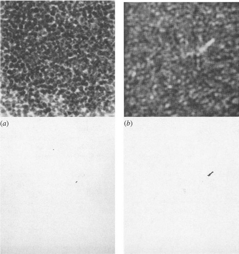
Figure 22.8 Foreign object detection in a packet of frozen vegetables (in this case sweet corn). (a) shows the original X-ray image, (b) shows an image in which texture analysis procedures have been applied to enhance any foreign objects, and (c) and (d) show the respective thresholded images. Notice the false alarms that are starting to arise in (c), and the increased confidence of detection of the foreign object in (d). For further details, see Patel et al. (1995).
Ultimately, the problem is difficult because the paradigm means of designing sensitive detectors—the matched filter—cannot be used, simply because of the high degree of variability in what has to be detected. With so many degrees of freedom—shape dimensions, size, intensity, texture, and so on—foreign objects can be highly difficult to detect successfully in complex images. Naturally, a lot depends on the nature of the substrate, and while a plain background might render the task trivial, a textured product substrate may make it impossible, or at least practically impossible in a real-time factory inspection milieu. In general, the solution devolves into not trying to detect the foreign object directly by means of carefully designed matched filters, but in trying to model the intensity pattern of the substrate with sufficient accuracy that any deviation due to the presence of a foreign object is detected and rendered visible. As hinted, the approach is to search for the unusual. Accordingly, the basic technique is to identify the 3σ or other appropriate points on all available measures and to initiate rejection when they are exceeded.
There is a fundamental objection to this procedure. If some limit (e.g., 3σ) is assumed, optimization cannot easily be achieved, since the proper method for achieving this is to find both the distributions—for the background substrate and for the foreign objects—and to obtain a minimum error decision boundary between them. (Ideally, this would be implemented in a multidimensional feature space appropriate to the task.) However, in this case we do not have the distribution corresponding to the foreign objects; we therefore have to fall back on “reasonable” acceptance limits based on the substrate distribution.
It might appear that this argument is flawed in that the proportion of foreign objects coming along the conveyor is well known. While it might occasionally be known, the levels of detectability of the foreign objects in the received images will be unknown and will be less than the actual occurrence levels. Hence, arriving at an optimal decision level will be very difficult.
A far worse problem often exists in practice. The occurrence rates for foreign objects might be almost totally unknown because of (1) their intrinsic variability and (2) their rarity. We might well ask, “How often will an elastic band fall onto a conveyor of peas?4”, but this is a question that is virtually impossible to answer. Maybe it is possible to answer somewhat more accurately the more general question of how often a foreign object of some sort will fall onto the conveyor, but even then the response may well be that somewhere between 1 in 100,000 and 1 in 10 million of bags of peas contain a foreign object. With low levels of risk, the probabilities are extremely difficult to estimate; indeed, there are few available data or other basis on which to calculate them. Consumer complaints can indicate the possible levels of risk, but they arise as individual items, and in any case many customers will not make any fuss and by no means all instances come to light.
With food products, the penalties for not detecting individual foreign objects are not usually especially great. Glass in baby food may be more apocryphal than real and may be unlikely to cause more than alarm. Similarly, small stones among the vegetables are more of a nuisance than a harm, though cracked teeth could perhaps result in litigation in the $2000 bracket. Far more serious are the problems associated with electric lamps, where a wire emerging from the solder pads is potentially lethal and is a substantive worry for the manufacturer. Litigation for deaths arising from this source could run to millions of dollars (corresponding to the individual’s potential lifetime earnings).
This discussion reveals that the cost rate2 rather than the error rate is the important parameter when there is even a remote risk to life and limb. Indeed, it concerned Rodd and his co-workers so much in relation to the inspection of electric lamps that they decided to develop special techniques for ensuring that their algorithms were tested sufficiently (Thomas and Rodd, 1994; Thomas et al., 1995). Computer graphics techniques were used to produce large numbers of images with automatically generated variations on the basic defects, and it was confirmed that the inspection algorithms would always locate them.
22.10 X-ray Inspection
In inspection applications, a tension exists between inspecting products early on, before significant value has been added to a potentially defective product, and at the end of the line, so that the quality of the final product is guaranteed. This consideration applies particularly with food products, where additives such as chocolate can be very expensive and constitute substantial waste if the basic product is broken or misshapen. In addition, inspection at the end of the line is especially valuable as oversized products (which may arise if two normal products become stuck together) can jam pack machines. Ideally, two inspection stations should be placed on the line in appropriate positions, but if only one can be afforded (the usual situation) it will generally have to be placed at the end of the line.
With many products, it is useful to be absolutely sure about the final quality as the customer will receive it. Thus, there is special value in inspecting the packaged products. Since the packets will usually be opaque, it will be necessary to inspect them under X-radiation. This results in significant expense, since the complete system will include not only the the X-ray source and sensing system but also various safety features including heavy shielding. As a result commercial X-ray food inspection systems rarely cost less than $60,000 and $200,000 is a more typical figure. Such figures do not take into account maintenance costs. It is also important to note that the X-ray source and the sensors deteriorate with time, so that sensitivity falls, and special calibration procedures have to be invoked.
Fortunately, the X-ray sensors can now take the form of linear photodiode packages constructed using integrated circuit technology.3 These packages are placed end to end to span the width of a food conveyor which may be 30 to 40 cm wide. They act as a line-scan camera that grabs images as the product moves along the conveyor. The main adjustments to be made in such a system are the voltage across the X-ray tube and the current passing through it. In food inspection applications, the voltage will be in the range of 30 to 100 kV, and the current will be in the range 3 to 10 mA. A basic commercial system will include thresholding and pixel counting, permitting the detection of small pieces of metal or other hard contaminants but not soft contaminants. In general, soft contaminants can be detected only if more sophisticated algorithms are used that examine the contrast levels over various regions of the image and arrive at a consensus that foreign objects are present—typically, with the help of texture analysis procedures.
The sensitivity of an X-ray detection system depends on a number of factors. Basically, it is highly dependent on the number of photons arriving at the sensors, and this number is proportional to the electron current passing through the X-ray tube. There are stringent rules on the intensities of X-radiation to which food products may be exposed, but in general these limits are not approached because of good sensitivity at moderate current levels. However, we shall not delve into these matters further here.
Sensitivity also depends critically on the voltages that are applied to X-ray tubes. It is well known that the higher the voltage, the higher the electron energies, the higher the energies of the resulting photons, and the greater the penetrating power of the X-ray beam. However, greater penetrating power is not necessarily an advantage, for the beam will tend to pass through the food without attenuation, and therefore without detecting any foreign objects. Although a poorly setup system may well be able to detect quite small pieces of metal without much trouble, detection of small stones and other hard contaminants will be less easy, and detection of soft contaminants will be virtually impossible. Thus, it is necessary to optimize the contrast in the input images.
Unfortunately, X-ray sources provide a wide range of wavelengths, all of which are scattered or absorbed to varying degrees by the intervening substances. In a thick sample, scattering can cause X-radiation to arrive at the detector after passing through material that is not in a direct line between the X-ray tube and the sensors. This makes a complete analysis of sensitivity rather complicated. In the following discussion we will ignore this effect and assume that the bulk of the radiation reaching the sensors follows the direct path from the X-ray source. We will also assume that the radiation is gradually absorbed by the intervening substances, in proportion to its current strength. Thus, we obtain the standard exponential formula for the decay of radiation through the material which we shall temporarily take to be homogeneous and of thickness z:
Here μ depends on the type of material and the penetrating power of the X-radiation. For monochromatic radiation of energy E, we have:
where ρ is the density of the material, A is its atomic weight, N is Avogadro’s number, a and b are numbers depending on the type of material, and kP and kC are decay constants resulting from photoelectric and Compton scattering, respectively (see e.g., Eisberg, 1961). It will not be appropriate to examine all the implications of this formula. Instead, we proceed with a rather simplified model that nevertheless shows how to optimize sensitivity:
Substituting in equation (22.10), we find:
If a minute variation in thickness or a small foreign object is to be detected sensitively, we need to consider the change in intensity resulting from a change in z or in αz. (Ultimately, it is the integral of μ dz that is important—see equation (22.10).) It will be convenient to relabel the latter quantity as a generalized distance X, and the inverse energy factor as f
The contrast due to the variation in generalized distance can now be expressed as:
This calculation shows that contrast should improve as the energy of the X-ray photons decreases. However, this result appears wrong, as reducing the photon energy will reduce the penetrating power, and in the end no radiation will pass through the sample. First, the sensors will not be sufficiently sensitive to detect the radiation. Specifically, noise (including quantization noise) will become the dominating factor. Second, we have ignored the fact that the X-radiation is not monochromatic. We shall content ourselves here with modeling the situation to take account of the latter factor. Assume that the beam has two energies, one fairly low (as above) and the other rather high and penetrating. This high-energy component will add a substantially constant value to the overall beam intensity and will result in a modified expression for the contrast:
To optimize sensitivity, we differentiate with respect to f:
When ![]() we have the previous result, that optimum sensitivity occurs for low E. However, when
we have the previous result, that optimum sensitivity occurs for low E. However, when ![]() , we have the result that optimum sensitivity occurs when E = X. In general, this formula gives an optimum X-ray that is above zero, in accordance with intuition. In passing, we note that graphical or iterative solutions of equation (22.21) are easily obtained.
, we have the result that optimum sensitivity occurs when E = X. In general, this formula gives an optimum X-ray that is above zero, in accordance with intuition. In passing, we note that graphical or iterative solutions of equation (22.21) are easily obtained.
Finally, we consider the exponential form of the signal given by equations (22.10), (22.13), and (22.14). These are nonlinear in X (i.e., αz), and meaningful image analysis algorithms would tend to require signals that are linear in the relevant physical quantity, namely, X. Thus, it is appropriate to take the logarithm of the signal from the input sensor, before proceeding with texture analysis or other procedures:
In this way, doubling the width of the sample doubles the change in intensity, and subsequent (e.g., texture analysis) algorithms can once more be designed on an intuitive basis. (In fact, there is a more fundamental reason for performing this transformation—that it performs an element of noise whitening, which should ultimately help to optimize sensitivity.)
22.11 The Importance of Color in Inspection
In many applications of machine vision, it is not necessary to consider color, because almost all that is required can be achieved using gray-scale images. For example, many processes devolve into shape analysis and subsequently into statistical pattern recognition. This situation is exemplified by fingerprint analysis and by handwriting and optical character recognition. However, there is one area where color has a big part to play. This is in the picking, inspection, and sorting of fruit. For example, color is very important in determining apple quality. Not only is it a prime indicator of ripeness, but it also contributes greatly to physical attractiveness and thus encourages purchase and consumption.
Whereas color cameras digitize color into the usual RGB (red, green, blue) channels, humans perceive color differently. As a result, it is better to convert the RGB representation to the HSI (hue, saturation, intensity) domain before assessing the colors of apples and other products.4 Space prevents a detailed study of the question of color; the reader is referred to more specialized texts for detailed information (e.g., Gonzalez and Woods, 1992; Sangwine and Horne, 1998). However, some brief comments will be useful. Intensity I refers to the total light intensity and is defined by:
Hue H is a measure of the underlying color, and saturation S is a measure of the degree to which it is not diluted by white light (S is zero for white light). S is given by the simple formula:
which makes it unity along the sides of the color triangle and zero for white light (R = G = B = 1). Note how the equation for S favors none of the R, G, B components. It does not express color but a measure of the proportion of color and differentiation from white.
Hue is defined as an angle of rotation about the central white point W in the color triangle. It is the angle between the pure red direction (defined by the vector R–W) and the direction of the color C in question (defined by the vector C–W). The derivation of a formula for H is fairly complex and will not be attempted here. Suffice it to say that it may be determined by calculating cos H, which depends on the dot product (C–W) • (R–W). The final result is:
 (22.26)
or 2π minus this value if B > G (Gonzalez and Woods, 1992).
When checking the color of apples, the hue is the important parameter. A rigorous check on the color can be achieved by constructing the hue distribution and comparing it with that for a suitable training set. The most straightforward way to carry out the comparison is to compute the mean and standard deviation of the two distributions to be compared and to perform discriminant analysis assuming Gaussian distribution functions. Standard theory (Section 4.5.3, equations (4.41) to (4.44)) then leads to an optimum hue decision threshold.
In the work of Heinemann et al. (1995), discriminant analysis of color based on this approach gave complete agreement between human inspectors and the computer following training on 80 samples and testing on another 66 samples. However, a warning about maintaining the lighting intensity levels identical to those used for training was given. In any such pattern recognition system, it is crucial that the training set be representative in every way of the eventual test set.
Full color discrimination would require an optimal decision surface to be ascertained in the overall 3-D color space. In general, such decision surfaces are hyperellipses and have to be determined using the Mahalanobis distance measure (see, for example, Webb, 2002). However, in the special case of Gaussian distributions with equal covariance matrices, or more simply with equal isotropic variances, the decision surfaces become hyperplanes.
22.12 Bringing Inspection to the Factory
The relationship between the producer of vision systems and the industrial user is more complex than might appear at first sight. The user has a need for an inspection system and states his need in a particular way. However, subsequent tests in the factory may show that the initial statement was inaccurate or imprecise. For example, the line manager’s requirements5 may not exactly match those envisaged by the factory management board. Part of the problem lies in the relative importance given to the three disparate functions of inspection mentioned earlier. Another lies in the change of perspective once it is seen exactly what defects the vision system is able to detect. It may be found immediately that one or more of the major defects that a product is subject to may be eliminated by modifications to the manufacturing process. In that case, the need for vision is greatly reduced, and the very process of trying out a vision system may end in its value being undermined and its not being taken up after a trial period. This does not detract from the inherent capability of vision systems to perform 100% untiring inspection and to help maintain strict control of quality. However, it must not be forgotten that vision systems are not cheap and that they can in some cases be justified only if they replace a number of human operators. Frequently, a payback period of two to three years is specified for installing a vision system.
Textural measurements on products are an attractive proposition for applications in the food and textile industries. Often textural analysis is written into the prior justification for, and initial specification of, an inspection system. However, what a vision researcher understands by texture and what a line inspector in either of these industries means by it tend to be different. Indeed, what is required of textural measurements varies markedly with the application. The vision researcher may have in mind higher-order6 statistical measures of texture, such as would be useful with a rough irregular surface of no definite periodicity7—as in the case of sand or pebbles on a beach, or grass or leaves on a bush. However, the textile manufacturer would be very sensitive to the periodicity of his fabric and to the presence of faults or overly large gaps in the weave. Similarly, the food manufacturer might be interested in the number and spatial distribution of pieces of pepper on a pizza, while for fish coatings (e.g., batter or breadcrumbs) uniformity will be important and “texture measurement” may end by being interpreted as determining the number of holes per unit area of the coating. Thus, texture may be characterized not by higher-order statistics but by rather obvious counting or uniformity checks. In such cases, a major problem is likely to be that of reducing the amount of computation to the lowest possible level, so that considerable expanses of fabric or large numbers of products can be checked economically at production rates. In addition, it is frequently important to keep the inspection system flexible by training on samples, so that maximum utility of the production line can be maintained.
With this backcloth to factory requirements, it is vital for the vision researcher to be sensitive to actual rather than idealized needs or the problem as initially specified. There is no substitute for detailed consultation with the line manager and close observation in the factory before setting up a trial system. Then the results from trials need to be considered very carefully to confirm that the system is producing the information that is really required.
22.13 Concluding Remarks
The number of relevant applications of computer vision to industrial tasks, and notably to automated visual inspection, is exceptionally high. For that reason, it has been necessary to concentrate on principles and methods rather than on individual cases. The repeated mention of hardware implementation has been necessary because the economics of real-time implementation is often the factor that ultimately decides whether a given system will be installed on a production line. However, processing speeds are also heavily dependent on the specific algorithms employed, and these in turn depend on the nature of the image acquisition system—including both the lighting and the camera setup. (The decision of whether to inspect products on a moving conveyor or to bring them to a standstill for more careful scrutiny is perhaps the most fundamental one for implementation.) Hence, image acquisition and realtime electronic hardware systems are the main topics of later chapters (Chapters 27 and 28).
More fundamentally, the reader will have noticed that a major purpose of inspection systems is to make instant decisions on the adequacy of products. Related to this purpose are the often fluid criteria for making such decisions and the need to train the system in some way, so that the decisions that are made are at least as good as those that would have arisen with human inspectors. In addition, training schemes are valuable in making inspection systems more general and adaptive, particularly with regard to change of product. Hence, the pattern recognition techniques of Chapter 24 are highly relevant to the process of inspection.
Ideally, the present chapter would have appeared after Chapters 24, chapter 27 and 28. However, it was felt that it was better to include it as early as possible, in order to maintain the reader’s motivation; also, Chapters 27 and 28 are perhaps more relevant to the implementation than to the rationale of image analysis.
On a different tack, it is worth noting that automated visual inspection falls under the general heading of computer-aided manufacture (CAM), of which computer-aided design (CAD) is another part. Today many manufactured parts can in principle be designed on a computer, visualized on a computer screen, made by computer-controlled (e.g., milling) machines, and inspected by a computer—all without human intervention in handling the parts themselves. There is much sense in this computer integrated manufacture (CIM) concept, since the original design dataset is stored in the computer, and therefore it might as well be used (1) to aid the image analysis process that is needed for inspection and (2) as the actual template by which to judge the quality of the goods. After all, why key in a separate set of templates to act as inspection criteria when the specification already exists on a computer? However, some augmentation of the original design information to include valid tolerances is necessary before the dataset is sufficient for implementing a complete CIM system. In addition, the purely dimensional input to a numerically controlled milling machine is not generally sufficient—as the frequent references to surface quality in the present chapter indicate.
Automated industrial inspection is a well-worn application area for vision that severely exercises the reliability, robustness, accuracy, and speed of vision software and hardware. This chapter has discussed the practicalities of this topic, showing how color and other modalities such as X-rays impinge on the basic vision techniques.
22.14 Bibliographical and Historical Notes
It is very difficult to provide a bibliography of the enormous number of papers on applications of vision in industry or even in the more restricted area of automated visual inspection. In any case, it can be argued that a book such as the present one ought to concentrate on principles and to a lesser extent on detailed applications and “mere” history. However, the review article by Newman and Jain (1995) gives a useful overview to 1995. For a review of PCB inspection, see Moganti et al. (1996).
The overall history of industrial applications of vision has been one of relatively slow beginnings as the potential for visual control became clear, followed only in recent years by explosive growth as methods and techniques evolved and as cost-effective implementations became possible as a result of cheaper computational equipment. In this respect, the year 1980 marked a turning point, with the instigation of important conferences and symposia, notably, that on “Computer Vision and Sensor-Based Robots” held at General Motors Research Laboratories during 1978 (see Dodd and Rossol, 1979), and the ROVISEC (Robot Vision and Sensory Controls) series of conferences organized annually by IFS (International Fluidic Systems) Conferences Ltd, UK, from 1981. In addition, useful compendia of papers (e.g., Pugh, 1983) and books outlining relevant principles and practical details (e.g., Batchelor et al., 1985) have been published. The reader is also referred to a special issue of IEEE Transactions on Pattern Analysis and Machine Intelligence (now dated) which is devoted to industrial machine vision and computer vision technology (Sanz, 1988).
Noble (1995) presents an interesting and highly relevant view of the use of machine vision in manufacturing. Davies (1995) develops the same topic by presenting several case studies together with a discussion of some major problems that remain to be addressed in this area.
The past few years have seen considerable interest in X-ray inspection techniques, particularly in the food industry (Boerner and Strecker, 1988; Wagner, 1988; Chan et al., 1990; Penman et al., 1992; Graves et al., 1994; Noble et al., 1994). In the case of X-ray inspection of food, the interest is almost solely in the detection of foreign objects, which could in some cases be injurious to the consumer. This has been a prime motivation for much work in the author’s laboratory (Patel et al., 1994, 1995; Patel and Davies, 1995).
Also of growing interest is the automatic visual control of materials such as lace during manufacture; in particular, high-speed laser scalloping of lace is set to become fully automated (King and Tao, 1995).
A cursory examination of inspection publications over the past few years reveals particular growth in emphasis on surface defect inspection, including color assessment, and X-ray inspection of bulk materials and baggage, (e.g., at airports). Two fairly recent journal special issues (Davies and Ip, eds., 1998; Nesi and Trucco, eds., 1999) cover defect inspection and include a paper on lace inspection (Yazdi, and King, 1998), while Tsai and Huang (2003) and Fish, et al. (2003) further emphasize the point regarding surface defects.
Work on color inspection includes both food (Heinemann et al., 1995) and pharmaceutical products (Derganc et al., 2003). Work on X-rays includes the location of foreign bodies in food (Patel et al., 1996; Batchelor et al., 2004), the internal inspection of solder joints (Roh et al., 2003), and the examination of baggage (Wang and Evans, 2003). Finally, a recent volume on inspection of natural products (Graves and Batchelor, 2003) has articles on inspection of ceramics, wood, textiles, food, live fish and pigs, and sheep pelts, and embodies work on color and X-ray modalities. In a sense, such work is neither adventurous nor glamorous. Indeed, it involves significant effort to develop the technology and software sufficiently to make it useful for industry—which means this is an exacting type of task, not tied merely to the production of academic ideas.
With time details often become less relevant, and the fundamental theory of vision limits what is practically possible in real applications. Hence, it does not seem fruitful to dwell further on applications here, beyond noting that the possibilities are continually expanding and should eventually cover most aspects of inspection, assembly automation, and vehicle guidance that are presently handled by humans. (Note, however, that for safety, legal, and social reasons, it may not be acceptable for machines to take control in all situations that they could theoretically handle.) Applications are particularly limited by available techniques for image acquisition and, as suggested above, by possibilities for cost-effective hardware implementation. For this reason,
1 On many food lines, g of packaging machines due to oversize products is one of the major problems.
2 The perceived cost rate may be even more important, and this can change markedly with reports appearing in the daily press.
3 The X-ray photons are first converted to visible light by passage through a layer of scintillating material.
4 Usually, a more important reason for use of HSI is to employ the hue parameter, which is independent of the intensity parameter, as the latter is bound to be particularly sensitive to lighting variations.
5 In many factories, line managers have the responsibility of maintaining production at a high level on an hour-by-hour basis, while at the same time keeping track of quality. The tension between these two aims, and particularly the underlying economic constraints, means that on occasion quality is bound to suffer.
6 The zero-order statistic is the mean intensity level. First-order statistics such as variance and skewness are derived from the histogram of intensities; second- and higher-order statistics take the form of gray-level co-occurrence matrices, showing the number of times particular gray values appear at two or more pixels in various relative positions. For more discussion on textures and texture analysis, see Chapter 26.
7 More rigorously, the fabric is intended to have a long-range periodic order that does not occur with sand or grass. There is a close analogy here with the long- and short-range periodic order for atoms in a crystal and in a liquid, respectively.