
CHAPTER 10 Circle Detection
10.1 Introduction
The location of round objects is important in many areas of image analysis, but it is especially important in industrial applications such as automatic inspection and assembly. In the food industry alone, a sizable proportion of products are round—biscuits, cakes, pizzas, pies, oranges, and so on (Davies, 1984c). In the automotive industry many circular components are used—washers, wheels, pistons, heads of bolts, and so on—while round holes of various sizes appear in such items as casings and cylinder blocks. In addition, buttons and many other everyday objects are round. All these manufactured parts need to be checked, assembled, inspected, and measured with high precision. Finally, objects can frequently be located by their holes, so finding round holes or features is part of a larger problem. Since round picture objects form a special category of their own, efficient algorithms should be available for analyzing digital images containing them. This chapter addresses some aspects of this problem.
An earlier chapter showed how objects may be found and identified using algorithms that involve boundary tracking (Table 10.1). Unfortunately, such algorithms are insufficiently robust in many applications; for example, they tend to be muddled by artifacts such as shadows and noise. This chapter shows that the Hough transform (HT) technique is able to overcome many ofthese problems. It is found to be particularly good at dealing with all sorts of difficulties, including quite severe occlusions. It achieves this capability not by adding robustness but by having robustness built in as an integral part of the technique.
Table 10.1 Procedure for finding objects using (r, θ) boundary graphs
| 1. Locate edges within the image. |
| 2. Link broken edges. |
| 3. Thin thick edges. |
| 4. Track around object outlines. |
| 5. Generate a set of (r, θ) plots. |
| 6. Match (r, θ) plots to standard templates. |
This procedure is not sufficiently robust with many types of real data (e.g., in the presence of noise, distortions in product shape, etc). In fact, it is quite common to find the tracking procedure veering off and tracking around shadows or other artifacts.
The application of the HT to circle detection is perhaps the most straightforward use of the technique. However, several enhancements and adaptations can be applied in order to improve the accuracy and speed of operation, and in addition to make the method work efficiently when detecting circles with a range of sizes. We will examine these modifications following a description of the basic HT techniques.
10.2 Hough-based Schemes for Circular Object Detection
In the original HT method for finding circles (Duda and Hart, 1972), the intensity gradient is first estimated at all locations in the image and is then thresholded to give the positions of significant edges. Then the positions of all possible center locations—namely, all points a distance R away from every edge pixel—are accumulated in parameter space, R being the anticipated circle radius. Parameter space can be a general storage area, but when looking for circles it is convenient to make it congruent to image space; in that case, possible circle centers are accumulated in a new plane of image space. Finally, parameter space is searched for peaks that correspond to the centers of circular objects. Since edges have nonzero width and noise will always interfere with the process of peak location, accurate center location requires the use of suitable averaging procedures (Davies, 1984c; Brown, 1984).
This approach requires that a large number of points be accumulated in parameter space, and so a revised form of the method has now become standard. In this approach, locally available edge orientation information at each edge pixel is used to enable the exact positions of circle centers to be estimated (Kimme et al., 1975). This is achieved by moving a distance R along the edge normal at each edge location. Thus, the number of points accumulated is equal to the number of edge pixels in the image.1 This represents a significant saving in computational load. For this saving to be possible, the edge detection operator that is employed must be highly accurate. Fortunately, the Sobel operator is able to estimate edge orientation to 1° and is very simple to apply (Chapter 5). Thus, the revised form of the transform is viable in practice.
As was seen in Chapter 5, once the Sobel convolution masks have been applied, the local components of intensity gradient gx and gy are available, and the magnitude and orientation of the local intensity gradient vector can be computed using the formulas:
Use of the arctan operation is not necessary when estimating center location coordinates (xc, yc) since the trigonometric functions can be made to cancel out:
the values of cos θ and sin θ being given by:
In addition, the usual edge thinning and edge linking operations—which normally require considerable amounts of processing—can be avoided if a little extra smoothing of the cluster of candidate center points can be tolerated (Davies, 1984c) (Table 10.2). Thus, this Hough-based approach can be a very efficient one for
Table 10.2 A Hough-based procedure for locating circular objects
| 1. Locate edges within the image. |
| 2. Link broken edges. |
| 3. Thin thick edges. |
| 4. For every edge pixel, find a candidate center point. |
| 5. Locate all clusters of candidate centers. |
| 6. Average each cluster to find accurate center locations. |
This procedure is particularly robust. It is largely unaffected by shadows, image noise, shape distortions, and product defects. Note that stages 1-3 of the procedure are identical to stages 1-3 in Table 10.1. However, in the Hough-based method, computation can be saved, and accuracy actually increased, by omitting stages 2 and 3.
locating the centers of circular objects, virtually all the superfluous operations having been eliminated, leaving only edge detection, location of candidate center points, and center point averaging to be carried out. It is also relevant that the method is highly robust in that if part of the boundary of an object is obscured or distorted, the object center is still located accurately. Some remarkable instances of this can be seen in Figs. 10.1 and 10.2. The reason for this useful property is clear from Fig. 10.3.
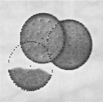
Figure 10.1 Location of broken and overlapping biscuits, showing the robustness of the center location technique. Accuracy is indicated by the black dots, which are each within 1/2 pixel of the radial distance from the center.
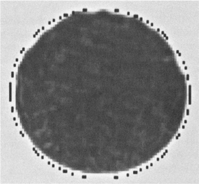
Figure 10.2 Location of a biscuit with a distortion, showing a chocolate-coated biscuit with excess chocolate on one edge. Note that the computed center has not been “pulled” sideways by the protuberances. For clarity, the black dots are marked 2 pixels outside the normal radial distance.
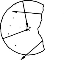
Figure 10.3 Robustness of the Hough transform when locating the center of a circular object. The circular part of the boundary gives candidate center points that focus on the true center, whereas the irregular broken boundary gives candidate center points at random positions.
This technique is so efficient that it takes slightly less time to perform the actual Hough transform part of the calculation than to evaluate and threshold the intensity gradient over the whole image. Part of the reason for these relative timings is that the edge detector operates within a 3 × 3 neighborhood and necessitates some 12 pixel accesses, four multiplications, eight additions, two subtractions, and an operation for evaluating the square root of sum of squares (equation (10.1)). As seen in Chapter 5, the latter type of operation is commonly approximated by taking a sum or maximum of absolute magnitudes of the component intensity gradients, in order to estimate the magnitude of the local intensity gradient vector:
However, this type of shortcut is not advisable in the present context, since an accurate value for the magnitude of this vector is required in order to compute the position of the corresponding candidate center location with sufficient precision. However, lookup tables provide a viable way around this problem.
Overall, the dictates of accuracy imply that candidate center location requires significant computation. However, substantial increases in speed are still possible by software means alone, as will be seen later in the chapter. Meanwhile, we consider the problems that arise when images contain circles of many different radii, or for one reason or another radii are not known in advance.
10.3 The Problem of Unknown Circle Radius
In a number of situations circle radius is initially unknown. One such situation is where a number of circles of various sizes are being sought—as in the case of coins, or different types of washers. Another is where the circle size is variable—as for food products such as biscuits—so that some tolerance must be built into the system. In general, all circular objects have to be found and their radii measured. In such cases, the standard technique is to accumulate candidate center points simultaneously in a number of parameter planes in a suitably augmented parameter space, each plane corresponding to one possible radius value. The centers of the peaks detected in parameter space give not only the location of each circle in two dimensions but also its radius. Although this scheme is entirely viable in principle, there are several problems in practice:
1. Many more points have to be accumulated in parameter space.
2. Parameter space requires much more storage.
3. Significantly greater computational effort is involved in searching parameter space for peaks.
To some extent this is to be expected, since the augmented scheme enables more objects to be detected directly in the original image.
We will shortly show that problems (2) and (3) may largely be eliminated by using just one parameter plane to store all the information for locating circles of different radii, that is, accumulating not just one point per edge pixel but a whole line of points along the direction of the edge normal in this one plane. In practice, the line need not be extended indefinitely in either direction but only over the restricted range of radii over which circular objects or holes might be expected.
Even with this restriction, a large number of points are being accumulated in a single parameter plane, and it might initially be thought that this would lead to such a proliferation of points that almost any “blob” shape would lead to a peak in parameter space might be interpreted as a circle center. However, this is not so, and significant peaks normally result only from genuine circles and some closely related shapes.
To understand the situation, consider how a sizable peak can arise at a particular position in parameter space. This can happen only when a large number of radial vectors from this position meet the boundary of the object normally. In the absence of discontinuities in the boundary, a contiguous set of boundary points can be normal to radius vectors only if they lie on the arc of a circle. (Indeed, a circle could be defined as a locus of points that are normal to the radius vector and that form a thin connected line.) If a limited number of discontinuities are permitted in the boundary, it may be deduced that shapes like that of a fan2 will also be detected using this scheme. Since it is in any case useful to have a scheme that can detect such shapes, the main problem is that there will be some ambiguity in interpretation—that is, does peak P in parameter space arise from a circle or a fan? In practice, it is quite straightforward to distinguish between such shapes with relatively little additional computation; the really important problem is to cut down the amount of computation needed to key into the initially unstructured image data. It is often a good strategy to prescreen the image to eliminate most of it from further detailed consideration and then to analyze the remaining data with tools having much greater discrimination. This two-stage template matching procedure frequently leads to significant savings in computation (VanderBrug and Rosenfeld, 1977; Davies, 1988i).
A more significant problem arises because of errors in the measurement of local edge orientation. As stated earlier, edge detection operators such as the Sobel introduce an inherent inaccuracy of about 1 °. Image noise typically adds a further 1 ° error, and for objects of radius 60 pixels the result is an overall uncertainty of about 2 pixels in the estimation of center location. This makes the scheme slightly less specific in its capability for detecting objects. In particular, edge pixels can now be accepted when their orientations are not exactly normal to the radius vector, and an inaccurate position will be accumulated in parameter space as a possible center point. Thus, the method may occasionally accept cams or other objects with a spiral boundary as potential circles.
Overall, the scheme is likely to accept the following object shapes during its prescreening stage, and the need for a further discrimination stage will be highly application-dependent:
If occlusions and breakages can be assumed to be small, then it will be safe to apply a threshold on peak size at, say, 70% of that expected from the smallest circle.3 In that case, it will be necessary to consider only whether the peaks arise from objects of types (1), (2), or (3). If, as usually happens, objects of types (2) or (3) are known not to be present, the method is immediately a very reliable detector of circles of arbitrary size. Sometimes specific rigorous tests for objects of types (2) and (3) will still be needed. They may readily be distinguished, for example, with the aid of corner detectors or from their radial intensity histograms (see Chapter 14 and 22).
Next, note that the information on radial distance has been lost by accumulating all votes in a single parameter plane. Hence, a further stage of analysis is needed to measure (or classify) object radius. This is so even if a stage of disambiguation is no longer required to confirm that the object is of the desired type. This extra stage of analysis normally involves negligible additional computation because the search space has been narrowed down so severely by the initial circle location procedure (see Figs. 10.4-10.6). The radial histogram technique already referred to can be used to measure the radius: in addition it can be used to perform a final object inspection function (see Chapter 22).
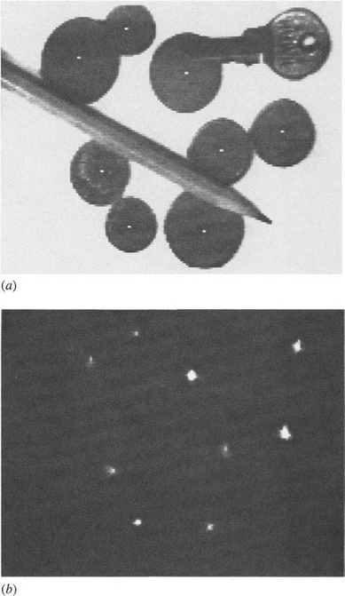
Figure 10.4 (a) Simultaneous location of coins and a key with the modified Hough scheme: the various radii range from 10 to 17 pixels; (b) transform used to compute the centers indicated in (a). Detection efficiency is unimpaired by partial occlusions, shape distortions, and glints. However, displacements of some centers are apparent. In particular, one coin (top left) has only two arcs showing. The fact that one of these is distorted, giving a lower curvature, leads to a displacement ofthe computed center. The shape distortions are due to rather uneven illumination.
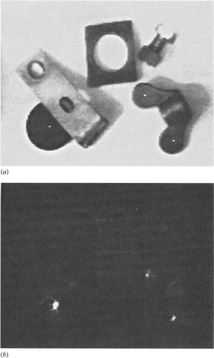
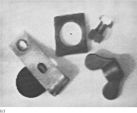
Figure 10.5 (a) Accurate simultaneous detection of a lens cap and a wing nut when radii are assumed to range from 4 to 17 pixels; (b) response in parameter space that arises with such a range of radii: note the overlap of the transforms from the lens cap and the bracket; (c) hole detection in the image of (a) when radii are assumed to fall in the range -26 to -9 pixels (negative radii are used since holes are taken to be objects of negative contrast). Clearly, in this image a smaller range of negative radii could have been employed.
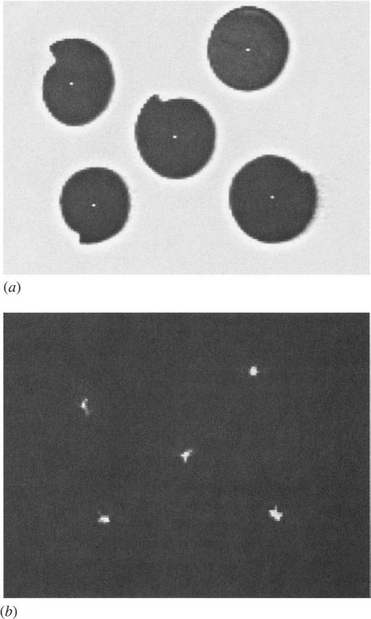
Figure 10.6 (a) Simultaneous detection of four (approximately) equiangular spirals and a circle of similar size (16 pixels radius), for assumed range of radii 9 to 22; (b) transform of (a). In the spiral with the largest step, the step size is about 6 pixels, and detection is possible only if some displacement of the center is acceptable. In such cases, the center is effectively the point on the evolute of the shape in parameter space that happens to have the maximum value. Note that cams frequently have shapes similar to those of the spirals shown here.
10.3.1 Experimental Results
The method described above works much as expected, the main problems arising with small circular objects (of radii less than about 20 pixels) at low resolution (Davies, 1988b). Essentially, the problems are those of lack of discrimination in the precise shapes of small objects (see Figs. 10.4-10.6), as anticipated earlier. More specifically, if a particular shape has angular deviations δψ relative to the ideal circular form, then the lateral displacement at the center of the object is rδψ. If this lateral displacement is 1 pixel or less, then the peak in parameter space is broadened only slightly and its height is substantially unchanged. Hence, detection sensitivity is similar to that for a circle. This model is broadly confirmed by the results of Fig. 10.6.
Theoretical analysis of the response can be carried out for any object by obtaining the shape of the evolute (envelope of the normals—see, for example, Tuckey and Armistead, 1953)—and determining the extent to which it spreads the peak in parameter space. However, performance is much as expected intuitively on the basis of the ideas already described, except that for small objects shape
discrimination is relatively poor. As suggested earlier, this can frequently be turned to advantage in that the method becomes a circular feature detector for small radii (see Fig. 10.5, where a wing nut is located).
Finally, objects are detected reliably even when they are partly occluded. However, occlusions can result in the centers of small objects being “pulled” laterally (Fig. 10.4)—a situation that seldom occurs with the original Hough scheme. When this is a problem in practical situations, it may be reduced by (1) cutting down the range of values of r that are employed in any one parameter plane (and hence using more than one plane), and (2) increasing resolution. Generally, subpixel accuracy of center location cannot be expected when a single-parameter plane is used to detect objects over a range of sizes exceeding a factor of about two. This is because of the amount of irrelevant “clutter” that appears in parameter space, which has the effect of reducing the signal-to-noise ratio (see Fig. 10.5). Similarly, attempting to find circular objects and holes simultaneously in the same parameter plane mitigates against good performance unless the sum of the ranges of radius values is restricted.
Thus, the approach outlined here involves a tradeoff between speed and accuracy. For high accuracy a relatively small range of values of r should be
employed in any one parameter plane, whereas for high speed one parameter plane will often cover the detection of all sizes of circles with sufficient accuracy. There is also the possibility of two-stage recognition (essentially an extension of the approach already outlined in Section 10.3) in order to find circles first with moderate and then with optimal accuracy.
These results using the modified Hough scheme confirm that we can locate objects of various radii within a parameter space of limited size. The scheme saves on storage requirements and on the amount of computation required to search parameter space for peaks, although it is not able to reduce the total number of votes that have to be accumulated in parameter space. A particular feature of the scheme is that it is essentially two-stage—the second stage being needed (when appropriate) for shape disambiguation and for size analysis. Two-stage procedures are commonly used to make image analysis more efficient, as will be seen in other chapters of this book (see especially Chapter 12 on ellipse detection).
10.4 The Problem of Accurate Center Location
The previous section analyzed the problem of how to cope efficiently with images containing circles of unknown or variable size. This section examines how circle centers may be located with high (preferably subpixel) accuracy. This problem is relevant because the alternative of increased resolution would entail the processing of many more pixels. Hence, attaining a high degree of accuracy with images of low or moderate resolution will provide an advantage.
There are several causes of inaccuracy in locating the centers of circles using the HT: (1) natural edge width may add errors to any estimates of the location of the center (this applies whether or not a thinning algorithm is employed to thin the edge, for such algorithms themselves impose a degree of inaccuracy even when noise is unimportant); (2) image noise may cause the radial position of the edge to become modified; (3) image noise may cause variation in the estimates of local edge orientation; (4) the object itself may be distorted, in which case the most accurate and robust estimate of the circle center is required (i.e., the algorithm should be able to ignore the distortion and take a useful average from the remainder of the boundary); (5) the object may appear distorted because of inadequacies in the method of illumination; and (6) the Sobel or other edge orientation operator will have a significant inherent inaccuracy of its own (typically 1°—see Chapter 5), which then leads to inaccuracy in estimating center location.
Evidently, it is necessary to minimize the effects of all these potential sources of error. In applying the HT, it is usual to remember that all possible center locations that could have given rise to the currently observed edge pixel should be accumulated in parameter space. Thus, we should accumulate in parameter space not a single candidate center point corresponding to the given edge pixel, but a point spread function (PSF) that may be approximated by a Gaussian error function. This will generally have different radial and transverse standard deviations. The radial standard deviation will commonly be 1 pixel—corresponding to the expected width of the edge—whereas the transverse standard deviation will frequently be at least 2 pixels, and for objects of moderate (60 pixels) radius the intrinsic orientation accuracy of the edge detection operator contributes at least 1 pixel to this standard deviation.
It would be convenient if the PSF arising from each edge pixel were isotropic. Then errors could initially be ignored and an isotropic error function could be convolved with the entire contents of parameter space, thus saving computation. However, this is not possible if the PSF is anisotropic, since the information on how to apply the local error function is lost during the process of accumulation.
When the center need only be estimated to within 1 pixel, these considerations hardly matter. However, when locating center coordinates to within 0.1 pixel, each PSF will have to contain 100 points, all of which will have to be accumulated in a parameter space of much increased spatial resolution, or its equivalent,4 if the required accuracy is to be attained. However, a technique is available that can cut down on the computation, without significant loss of accuracy, as will be seen below.
10.4.1 Obtaining a Method for Reducing Computational Load
The HT scheme outlined here for accurately locating circle centers is a completely parallel approach. Every edge pixel is examined independently, and only when this process is completed is a center looked for. Since there is no obvious means of improving the underlying Hough scheme, a sequential approach appears to be required if computation is to be saved. Unfortunately, sequential methods are often less robust than parallel methods. For example, an edge tracking procedure can falter and go wandering off, following shadows and other artifacts around the image. In the current application, if a sequential scheme is to be successful in the sense of being fast, accurate, and robust, it must be subtly designed and retain some of the features of the original parallel approach. The situation is now explored in more detail.
First, note that most of the inaccuracy in calculating the position of the center arises from transverse rather than radial errors. Sometimes transverse errors can fragment the peak that appears in the region of the center, thereby necessitating a
considerable amount of computation to locate the real peak accurately. Thus, it is reasonable to concentrate on eliminating transverse errors.
This immediately leads to the following strategy: find a point D in the region of the center and use it to obtain a better approximation A to the center by moving from the current edge pixel P a distance equal to the expected radius r in the direction of D (Fig. 10.7). Then repeat the process one edge pixel at a time until all edge pixels have been taken into account. Although intuition indicates that this strategy will lead to a good final approximation to the center, the situation is quite complex. There are two important questions:
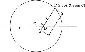
There is a small range of boundary pixels for which the method described here gives a location A that is worse than the initial approximation D (see Fig. 10.8). However, this does not mean that our intuition is totally wrong, and theory confirms the usefulness of the approach when d is small (d « r). Figure 10.9 shows a set of graphs that map out the loci of points forming second approximations to the center positions for initial approximations at various distances d from the center. In each graph the locus is that obtained on moving around the periphery of the circle. Generally, for small d it is seen that the second approximation is on average a significantly better approximation than the initial approximation. Theory shows that for small d the mean result will be an improvement by a factor close to 1.6 (the limiting value as d → 0is π/2 (Davies, 1988e)). In order to prove this result, it is first necessary to show that as d approaches zero, the shape of the locus becomes a circle whose center is halfway between the original approximation D and the center C, and whose radius is d/2 (Fig. 10.9).
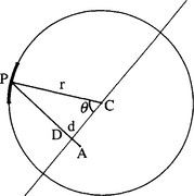
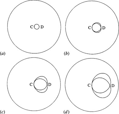
Figure 10.9 Loci obtained for various starting approximations: (a) d = 0.17r;(b) d = 0.32r; (c) d = 0.50r;(d) d = 0.68r.
At first, an improvement factor of only ∼ 1.6 seems rather insignificant—until it is remembered that it should be obtainable for every circle boundary pixel. Since there are typically 200 to 400 such pixels (e.g., for r ![]() 50), the overall improvement
50), the overall improvement
can in principle be virtually infinite. (Limitations on the actual accuracy are discussed later in this chapter.) However, to maximize the gain in accuracy, the order in which the algorithm processes boundary pixels should be randomized. (If this were not done, two adjacent pixels might often appear consecutively, the second giving negligible additional improvement in center location.)
10.4.2 Improvements on the Basic Scheme
In practice, convergence initially occurs much as theory suggests it does. However, after a time no further improvement occurs, and the system settles down to a situation where it is randomly wandering around the ideal center, sometimes getting better and sometimes getting worse. The reason for this is that the particular approximation obtained at this stage depends more on the noise on individual edge pixels than on the underlying convergence properties discussed above.
To improve the situation further, the noise on the edge pixels must be suppressed by an averaging procedure. Since the positions of the successive approximations produced by this method after a certain stage are essentially noise limited, the best final approximation will result from averaging all the individual approximations by accumulating all the intermediate x and y values and finding the means. Furthermore, just as the best final approximation is obtained by averaging, so the best intermediate approximations are obtained by a similar averaging process—in which the x and y values so far accumulated are divided by the current number. Thus, at this stage of the algorithm it is not necessary to use the previously calculated position at the starting point for the next approximation, but rather some position derived from it. If the kth position that is accumulated is (uk, vk), then the kth best estimate is given by:
Typically, 400 boundary pixels are available, each of which gives an independent measurement of position. On balance we would expect each of the component (x and y) inaccuracies to be averaged and thereby reduced by a factor of ![]() (Davies, 1987h). Hence, the linear accuracy should improve from around 1 pixel to around 0.1 pixel.
(Davies, 1987h). Hence, the linear accuracy should improve from around 1 pixel to around 0.1 pixel.
There are three stages of calculation in the algorithm:
1. Find the position of the center to within 2 pixels by the usual Hough technique.
2. Use the procedure as originally outlined until it settles down with an accuracy of 0.5 pixel—that is, until it is limited by radial errors rather than basic convergence problems.
3. Use the averaging version of the procedure (equation (10.9) and equation (10.10)) to obtain the final result, with an accuracy of 0.1 pixel.
In practice, it is possible to eliminate stage 2, with stage 1 then being used to get within 1 pixel of the center and stage 3 to get down to 0.1 pixel of the center. To retain robustness and accuracy, most of the work is done by parallel processing procedures (stage 1) or procedures that emulate parallel processing (stage 3).
To confirm that stage 3 emulates parallel processing, note that if a set of random points near the center were chosen as initial approximations, then a parallel procedure could be used to accumulate a new set of better approximations to the center, by using radial information from each of the edge pixels. However, the actual stage 3 is better than this as it uses the current best estimate of the position of the center as the starting position for each approximation. This is possible only ifthe calculation is being done sequentially rather than in parallel. Such a method is an improvement only if it is known that the initial approximation is good enough and if edge pixels that disagree badly with the currently known position of the center can be discarded as being due, for example, to a nearby object. A mechanism has to be provided for this eventuality within the algorithm. A useful strategy is to eliminate from consideration those edge pixels that would on their own point to center locations further than 2 pixels from the approximation indicated by stage 1.
10.4.3 Discussion
Based on the forgoing description, we might conclude that instead of using a successive approximation approach we could continue to use the same initial approximation for all boundary pixels and then average the results at the end. This would not be valid, however, since a fixed bias of 0.64d in an unknown direction would then result and there would be no way of removing it. Thus, the only real options are a set of random starting approximations or the sequence of approximations outlined above.
One thing that would upset the algorithm would be the presence of gross occlusions in the object, making less than about 30% of it visible, so that the center position might be known accurately in one direction but would be uncertain in a perpendicular direction. Unfortunately, such uncertainties would not be apparent with this method, since the absence of information might well lead to little transverse motion of the apparent center, which would then retain the same incorrect position.
10.4.4 Practical Details
The basis of the algorithm for improving on an approximation D (xi, yi) to a circle of center C is that of moving a distance r from a general boundary pixel P (x, y) in
This process is computationally efficient, since it does not require the evaluation of any trigonometric functions—the most complex operations involved being the calculation of various ratios and the evaluation of a square root.
Generally, it is apparently adequate to randomize boundary pixels (see Section 10.3) by treating them cyclically in the order they appear in a normal raster scan of the image, and then processing every nth one5 until all have been used (Davies, 1988e). The number n will normally be in the range 50-150 (or for general circles with N boundary pixels, take n ![]() NMore Detailed Estimates of Speed/4). One advantage of randomizing boundary pixels is that processing can be curtailed at any stage when sufficient accuracy has been attained, thereby saving computation. This technique is particularly valuable in the case of food products such as biscuits, where accuracy is generally not as much of a problem as speed of processing.
NMore Detailed Estimates of Speed/4). One advantage of randomizing boundary pixels is that processing can be curtailed at any stage when sufficient accuracy has been attained, thereby saving computation. This technique is particularly valuable in the case of food products such as biscuits, where accuracy is generally not as much of a problem as speed of processing.
The algorithm is straightforward to set up, parameters being adjusted on a heuristic basis rather than adhering to any specific theory. This does not seem to lead to any real problems or to compromise accuracy. The results of center finding seem to be generally within 0.1 to 0.2 pixel (see below) for accurately made objects where such measurements can meaningfully be made. This rarely applies to food products such as biscuits, which are commonly found to be circular to a tolerance of only 5 to 10%.
When the algorithm was tested using an accurately made dark metal disc, accuracy was found to be in the region of 0.1 pixel (Davies, 1988e). However, some difficulty arose because of uncertainty in the actual position of the center. A slight skewness in the original image was found to contribute to such location errors—possibly about 0.05 pixel in this case. The reason for the skewness appeared to lie in a slight nonuniformity in the lighting of the metal disc. It became clear that it will generally be difficult to eliminate such effects and that 0.1-pixel accuracy is close to the limit of measurement with such images. However, other tests using simulated (accurate) circles showed that the method has an intrinsic accuracy of better than 0.1 pixel.
Other improvements to the technique involve weighting down the earlier, less accurate approximations in obtaining the average position of the center. Weighting down can be achieved by the heuristic of weighting approximations in proportion to their number in the sequence. This strategy seems capable of finding center locations within 0.05 pixel—at least for cases where radii are around 45 pixels and where some 400 edge pixels are providing information about the position of each center. Although accuracy is naturally data-dependent, the approach fulfills the specification originally set out—of locating the centers of circular objects to 0.1 pixel or better, with minimal computation. As a by-product of the computation, the radius r can be obtained with exceptionally high accuracy—generally within 0.05 pixel (Davies, 1988e).
10.5 Overcoming the Speed Problem
The previous section studied how the accuracy of the HT circle detection scheme could be improved substantially, with modest additional computational cost. This section examines how circle detection may be carried out with significant improvement in speed. There is a definite tradeoff between speed and accuracy, so that greater speed inevitably implies lower accuracy. However, at least the method to be adopted permits graceful degradation to take place.
One way to overcome the speed problem described in Section 10.2 is to sample the image data; another is to attempt to use a more rudimentary type of edge detection operator; and a third is to try to invent a totally new strategy for center location.
Sampling the image data tends to mean looking at, say, every third or fourth line, to obtain a speed increase by a factor of three or so. However, improvements beyond this are unlikely, for we would then be looking at much less of the boundary of the object and the method would tend to lose its robustness. An overall improvement in speed by more than an order of magnitude appears to be unattainable.
Using a more rudimentary edge detection operator would necessarily give much lower accuracy. For example, the Roberts cross operator (Roberts, 1965) could be used, but then the angular accuracy would drop by a factor of five or so (Abdou and Pratt, 1979), and in addition the effects of noise would increase markedly so that the operator would achieve nowhere near its intrinsic accuracy. With the Roberts cross operator, noise in any one of the four pixels in the neighborhood will make estimation of orientation totally erroneous, thereby invalidating the whole strategy of the center finding algorithm.
In this scenario Davies (1987) attempted to find a new strategy that would have some chance of maintaining the accuracy and robustness of the original approach, while improving speed by at least an order of magnitude. In particular, it would be useful to aim for improvement by a factor of three by sampling and by another factor of three by employing a very small neighborhood. By opting for a 2-element neighborhood, the capability of estimating edge orientation is lost. However, this approach still permits an alternative strategy based on bisecting horizontal and vertical chords of a circle. This approach requires two passes over the image to determine the center position fully. A similar amount of computation is needed as for a single application of a 4-element neighborhood edge detector, so it should be possible to gain the desired factor of three in speed relative to a Sobel operator via the reduced neighborhood size. Finally, the overall technique involves much less computation, the divisions, multiplications, and square root calculations being replaced by 2-element averaging operations, thereby giving a further gain in speed. Thus, the gain obtained by using this approach could be appreciably over an order of magnitude.
10.5.1 More Detailed Estimates of Speed
This section presents formulas from which it is possible to estimate the gain in speed that would result by applying the above strategy for center location. First, the amount of computation involved in the original Hough-based approach is modeled by:
T0 = the total time taken to run the algorithm on an N × N pixel image
s = the time taken per pixel to compute the Sobel operator and to threshold the intensity gradient g
S = the number of edge pixels that are detected
t0 = the time taken to compute the position of a candidate center point.
Next, the amount of computation in the basic chord bisection approach is modeled as
T = the total time taken to run the algorithm
q = the time taken per pixel to compute a 2-element x or y edge detection operator and to perform thresholding
Q = the number of edge pixels that are detected in one or other scan direction
t = the time taken to compute the position of a candidate center point coordinate (either xc or yc).
In equation (10.15), the factor of two results because scanning occurs in both horizontal and vertical directions. If the image data are now sampled by examining only a proportion α of all possible horizontal and vertical scan lines, the amount of computation becomes:
The gain in speed from using the chord bisection scheme with sampling is therefore:
Typical values of relevant parameters for, say, a biscuit of radius 32 pixels in a 128 × 128 pixel image are:
This is a substantial gain, and we now consider more carefully how it could arise. If we assume N » S, Q, we get:
This is obviously the product of the sampling factor l/α and the gain from applying an edge detection operator twice in a smaller neighborhood (i.e., applied both horizontally and vertically). In the above example, l/α = 3 and s/2q = 3, this figure resulting from the ratio of the numbers of pixels involved. This would give an ideal gain of 9, so the actual gain in this case is not much changed by the terms in t0 and t.
It is important that the strategy also involves reducing the amount of computation in determining the center from the edge points that are found. However, in all cases the overriding factor involved in obtaining an improvement in speed is the sampling factor l/α. If this factor could be improved further, then significant additional gains in speed could be obtained—in principle without limit, but in practice the situation is governed by the intrinsic robustness of the algorithm.
10.5.2 Robustness
Robustness can be considered relative to two factors: the amount of noise in the image; and the amount of signal distortion that can be tolerated. Fortunately, both the original HT and the chord bisection approach lead to peak finding situations. If there is any distortion of the object shape, then points are thrown into relatively random locations in parameter space and consequently do not have a significant direct impact on the accuracy of peak location. However, they do have an indirect impact in that the signal-to-noise ratio is reduced, so that accuracy is impaired. Ifa fraction β of the original signal is removed, leaving a fraction γ = 1—β, due either to such distortions or occlusions or to the deliberate sampling procedures already outlined, then the number of independent measurements of the center location drops to a fraction γ of the optimum. Thus, the accuracy of estimation of the center location drops to a fraction ![]() of the optimum. Since noise affects the optimum accuracy directly, we have in principle shown the result of both major factors governing robustness.
of the optimum. Since noise affects the optimum accuracy directly, we have in principle shown the result of both major factors governing robustness.
The important point here is that the effect of sampling is substantially the same as that of signal distortion, so that the more distortion that must be tolerated, the higher the value α has to have. This principle applies both to the original Hough approach and to the chord bisection algorithm. However, the latter does its peak finding in a different way—via 1-D rather than 2-D averaging processes. As a result, it turns out to be somewhat more robust than the standard HT in its capability for accepting a high degree of sampling.
This gain in capability for accepting sampling carries with it a set of related disadvantages: highly textured objects may not easily be located by the method; high noise levels may muddle it via the production of too many false edges; and (since it operates by specific x and y scanning mechanisms) there must be a sufficiently small amount of occlusion and other gross distortion that a significant number of scans (both horizontally and vertically) pass through the object. Ultimately, then, the method will not tolerate more than about one-quarter of the circumference of the object being absent.
10.5.3 Experimental Results
Tests (Davies, 1987l) with the image in Fig. 10.10 showed that gains in speed of more than 25 can be obtained, with values of α down to less than 0.1 (i.e., every tenth horizontal and vertical line scanned). To obtain the same accuracy and reliability with smaller objects, a larger value of α was needed. This can be viewed as keeping the number of samples per object roughly constant. The maximum gain in speed was then by a factor of about 10. The results for broken circular products (Fig. 10.11 and 10.12) are self-explanatory; they indicate the limits to which the method can be taken and confirm that it is straightforward to set the algorithm up by eye. An outline of the complete algorithm is given in Fig. 10.14.
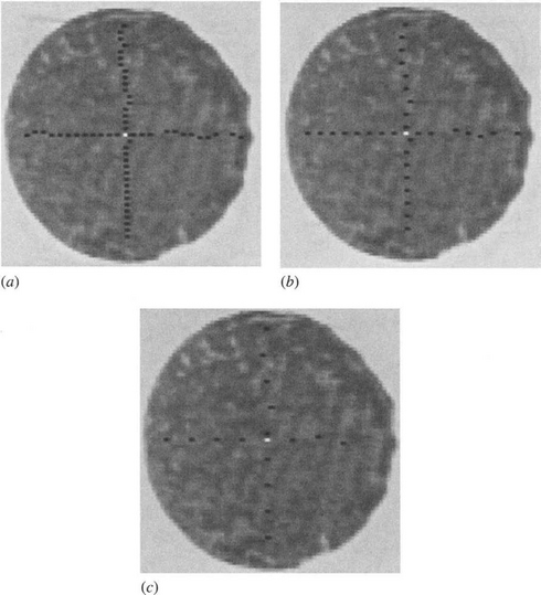
Figure 10.10 Successful object location using the chord bisection algorithm for the same initial image, using successive step sizes of 2, 4, and 8 pixels. The black dots show the positions of the horizontal and vertical chord bisectors, and the white dot shows the position found for the center.
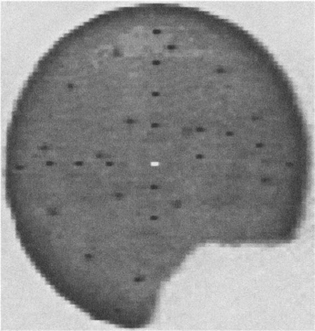
Figure 10.11 Successful location of a broken object using the chord bisection algorithm: only about one-quarter of the ideal boundary is missing.
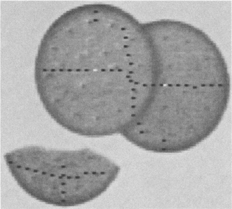
Figure 10.12 A test on overlapping and broken biscuits: the overlapping objects are successfully located, albeit with some difficulty, but there is no chance of finding the center of the broken biscuit since over one-half of the ideal boundary is missing.
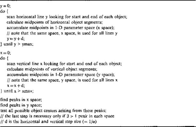
Figure 10.13 shows the effect of adjusting the threshold in the 2-element edge detector. The result of setting it too low is seen in Fig. 10.13a. Here the surface texture of the object has triggered the edge detector, and the chord midpoints give rise to a series of false estimates of the center coordinates. Figure 10.13b shows the result of setting the threshold at too high a level, so that the number of estimates of center coordinates is reduced and sensitivity suffers. The images in Fig. 10.10 were obtained with the threshold adjusted intuitively, but its value is nevertheless close to the optimum. However, a more rigorous approach can be taken by optimizing a suitable criterion function. There are two obvious functions: (1) the number of accurate center predictions n; and (2) the speed-sensitivity product. The speed-sensitivity product can be written in the form ![]() , where T is the execution time (the reason for the square root being as in Section 10.4.2). The two methods of optimization make little difference in the example of Fig. 10.13. However, had there
, where T is the execution time (the reason for the square root being as in Section 10.4.2). The two methods of optimization make little difference in the example of Fig. 10.13. However, had there
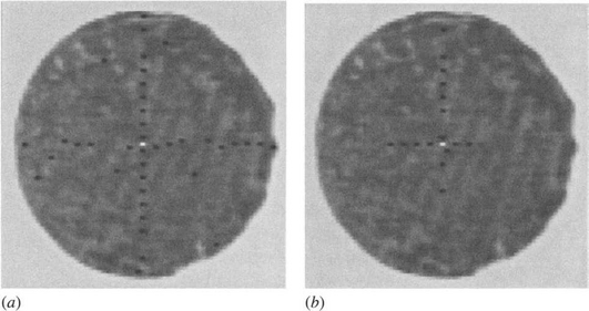
Figure 10.13 Effect of misadjustment of the gradient threshold: (a) effect of setting the threshold too low, so that surface texture muddles the algorithm; (b) loss of sensitivity on setting the threshold too high.
been a strong regular texture on the object, the situation would have been rather different.
10.5.4 Summary
The center location procedure described in this chapter is normally over an order of magnitude faster than the standard Hough-based approach. Typically,
execution times are reduced by a factor of ∼25. In exacting real-time applications, this may be important, for it could mean that the software will operate without special-purpose hardware accelerators. Robustness is good both in noise suppression capability and in the ability to negotiate partial occlusions and breakages of the object being located. The method tolerates at least one-quarter of the circumference of an object being absent for one reason or another. Although this is not as good as for the original HT approach, it is adequate for many real applications. In addition, it is entirely clear on applying the method to real image data whether the real image data would be likely to muddle the algorithm—since a visual indication of performance is available as an integral part of the method.
Robustness is built into the algorithm in such a way as to emulate the standard Hough-based approach. It is possible to interpret the method as being itself a Hough-based approach, since each center coordinate is accumulated in its own 1-D “parameter space.” These considerations give further insight into the robustness of the standard Hough technique.
10.6 Concluding Remarks
Although the Hough technique has been found to be effective and highly robust against occlusions, noise, and other artifacts, it incurs considerable storage and computation—especially if it is required to locate circles of unknown radius or if high accuracy is required. Techniques have been described whereby the latter two problems can be tackled much more efficiently. In addition, a method has been described for markedly reducing the computational load involved in circle detection. The general circle location scheme is a type of HT, but although the other two methods are related to the HT, they are distinct methods that draw on the HT for inspiration. As a result, they are rather less robust, although the degree of robustness is quite apparent and there is little risk of applying them when their use would be inappropriate. As remarked earlier, the HT achieves robustness as an integral part of its design. This is also true of the other techniques described, for which considerable care has been taken to include robustness as an intrinsic part of the design rather than as an afterthought.
As in the case of line detection, a trend running through the design of circle detection schemes is the deliberate splitting of algorithms into two or more stages. This consideration is useful for keying into the relevant parts of an image prior to finely discriminating one type of object or feature from another, or prior to measuring dimensions or other characteristics accurately. The concept can be taken further, in that all the algorithms discussed in this chapter have improved their efficiency by searching first for edge features in the image. The concept of two-stage template matching is therefore deep-seated in the methodology of the subject and is developed further in later chapters—notably those on ellipse and corner detection. Although two-stage template matching is a standard means of increasing efficiency (VanderBrug and Rosenfeld, 1977; Davies, 1988i), it is not at all obvious that it is always possible to increase efficiency by this means. It appears to be in the nature of the subject that ingenuity is needed to discover ways of achieving this efficiency.
The Hough transform is straightforwardly applied to circle detection. This chapter has demonstrated that its robustness is impressive in this case, though there are other relevant practical issues such as accuracy, speed, and storage requirements—some of which can be improved by employing parameter spaces of reduced dimension.
10.7 Bibliographical and Historical Notes
The Hough transform was developed in 1962 and first applied to circle detection by Duda and Hart (1972). However, the now standard HT technique, which makes use of edge orientation information to reduce computation, only emerged three years later (Kimme et al., 1975). Davies’ work on circle detection for automated inspection required real-time implementation and also high accuracy. This spurred the development of the three main techniques described in Sections 10.3-10.5 of this chapter (Davies, 1987l, 1988b,e). In addition, Davies has considered the effect of noise on edge orientation computations, showing in particular their effect in reducing the accuracy of center location (Davies, 1987k).
Yuen, et al. (1989) reviewed various existing methods for circle detection using the HT. In general, their results confirmed the efficiency of the method of Section 10.3 for unknown circle radius, although they found that the two-stage process involved can sometimes lead to slight loss of robustness. It appears that this problem can be reduced in some cases by using a modified version of the algorithm of Gerig and Klein (1986). Note that the Gerig and Klein approach is itself a two-stage procedure: it is discussed in detail in the next chapter. More recently, Pan et al. (1995) have increased the speed of computation of the HT by prior grouping of edge pixels into arcs, for an underground pipe inspection application.
The two-stage template matching technique and related approaches for increasing search efficiency in digital images were known by 1977 (Nagel and Rosenfeld, 1972; Rosenfeld and VanderBrug, 1977; VanderBrug and Rosenfeld, 1977) and have undergone further development since then—especially in relation to particular applications such as those described in this chapter (Davies, 1988i).
Most recently, Atherton and Kerbyson (1999) (see also Kerbyson and Atherton, 1995) showed how to find circles of arbitrary radius in a single parameter space using the novel procedure of coding radius as a phase parameter and then performing accumulation with the resulting phase-coded annular kernel. Using this approach, they attained higher accuracy with noisy images. Goulermas and Liatsis (1998) showed how the Hough transform could be fine-tuned for the detection of fuzzy circular objects such as overlapping bubbles by using genetic algorithms. In effect, genetic algorithms are able to sample the solution space with very high efficiency and hand over cleaner data to the following Hough transform. Toennies et al. (2002) showed how the Hough transform can be used to localize the irises of human eyes for real-time applications, one advantage of the transform being its capability for coping with partial occlusion—a factor that is often quite serious with regard to the iris.
10.8 Problems
1. Prove the result of Section 10.4.1, that as D approaches C and d approaches zero (Fig. 10.9), the shape of the locus becomes a circle on DC as diameter.
1. (a) Describe the use of the Hough transform for circular object detection, assuming that object size is known in advance. Show also how a method for detecting ellipses could be adapted for detecting circles of unknown size.
(b) A new method is suggested for circle location which involves scanning the image both horizontally and vertically. In each case, the midpoints of chords are determined and their x or y coordinates are accumulated in separate 1-D histograms. Show that these can be regarded as simple types of Hough transform, from which the positions of circles can be deduced. Discuss whether any problems would arise with this approach; consider also whether it would lead to any advantages relative to the standard Hough transform for circle detection.
(c) A further method is suggested for circle location. This again involves scanning the image horizontally, but in this case, for every chord that is found, an estimate is immediately made of the two points at which the center could lie, and votes are placed at those locations. Work out the geometry of this method, and determine whether it is faster than the method outlined in (b). Determine whether the method has any disadvantages compared with the method in (b).
1 We assume that objects are known to be either lighter or darker than the background, so that it is only necessary to move along the edge normal in one direction.
2 In this chapter all references to “fan” mean a four-blade fan shape bounded by two concentric circles with eight equally spaced radial lines joining them.
3 Note, however, that size-dependent effects can be eliminated by appropriate weighting of the votes cast at different radial distances.
4 For example, some abstract list structure might be employed that effectively builds up to high resolution only where needed (see also the adaptive HT scheme described in Chapter 11).
5 The final working algorithm is slightly more complex. If the nth pixel has been used, take the next one that has not been used. This simple strategy is sufficiently random and also overcomes problems of n sometimes being a factor of N.