2.2. The Estimation of Computational Complexity

Search in book...
Toggle Font Controls
Create new playlist

Name your new playlist

Playlist description (optional)
Sign In

Email address

Password

Forgot Password?

or

Continue with Facebook

Continue with Google
Sign Up

Full Name

Email address

Confirm Email Address

Password

or

Continue with Facebook

Continue with Google

2.2. The Estimation of Computational Complexity

The aim of this section is to estimate the computational complexity, based on the mathematical model presented in Chapter 1, when the multi-granular computing is used (Zhang and Zhang, 1990d, 1992).

2.2.1. The Assumptions

A problem space is assumed to be a finite set. Symbol

denotes the number of elements in X. Sometimes, we simply use X instead of

if no confusion is made.

If we solve the problem X directly, i.e., finding a goal in X, the computational complexity is assumed to be

. Then, the complexity will be changed to

by using the multi-granular computing. Now, the point is in what conditions that we may have the result

Before the discussion, we make the following assumption for

Hypothesis A

Assume that

only depends on the number of elements in X, and independent of its structure, or other attributes. Both domain and range of

are assumed to be

, i.e., a non-negative real number. Namely,

(1)

is a monotonically increasing function on

(2)

, we have

is called a computational complexity function on X, or complexity function for short.

Now, we solve X by using the multi-granular computing strategy. That is, X is classified with respect to

. Its corresponding quotient space is denoted by

. Then the original problem on X is converted into the corresponding problem on

. Since some information will lose on

due to the abstraction, generally, we can't find the goal of X directly from its quotient space

. Instead, we can only have a useful clue to the final solution of X from

. Thus, in order to describe the relation between the results obtained from the quotient and its original spaces, we introduce a new function as follows.

Definition 2.1

Assume that

is a quotient space of X and f is a complexity function of X. Suppose that the complexity function of

is less than

and the number of elements which might contain the goal is estimated at g at most. Define a goal estimation function

as follows:

Assume that

is a monotonically increasing function and

We have a sequence

of quotient spaces with t levels, where

is a quotient space of

. After the multi-granular computing with t levels, the total complexity function is assumed to be

. We next estimate the

2.2.2. The Estimation of the Complexity Under Deterministic Models

Our goal is to estimate the asymptotic property of complexity function under the multi-granular computing. For simplicity, let

, i.e., X has

elements. The other variables are limited to the order of

, and

, where

Local Partition Method

Definition 2.2

Assume

. The complexity function

is called divergent if for any given b > 0, have

Case

Suppose that

is a quotient space of X. We seek the goal of X from

. When solving the problem on

, the computational complexity only depends on the number of elements in

. After the amount

of computation, we find element

which might contain the goal. Due to

, there is only one such element,

. Again, assume that each equivalence class has the same number of elements.

Then, we seek the goal within the equivalence class

(

is an element in X₁) in X.

When

, from

we have

. Thus, the total computational complexity for solving X by the multi-granular computing with two levels is

(2.1)

Regarding

as a set of X, if set

is too large, then

is further partitioned. Assume that

is a quotient set of set

and

The total complexity for solving X by the multi-granular computing with three levels is

(2.2)

where,

is an element of

which might contain the goal.

From induction, the total complexity for solving X by the multi-granular computing with t levels is

(2.3)

where

If in each level, its elements are classified into c equivalence classes without exception, where

is an integer, i.e.,

. Since

, we have

, where

. Then, we have

. Substituting

into (2.3), we have

, i.e.,

We have the following proposition.

Proposition 2.1

If a unique element which contains the goal can be found at each granular level, i.e.,

, there exists a hierarchical partition method for X such that X can be solved in a linear time (

), in spite of the form of complexity function f(X) (f(X) might be divergent).

Example 2.4

We are given

coins, one of which is known to be lighter than the rest. Using a two-pan scale, we must find the counterfeit coin as soon as possible.

To solve the problem, we may weigh a pair of coins (one in each pan) at a time. That is, we find the counterfeit one from

coins directly. The mean computational complexity, the average number of weighing, is

. By the multi-granular computing,

coins may first be divided into three groups equally. Then a quotient space

is gained. Obviously, we can find which group will contain the counterfeit coin in one test. That is, by weighing A and B, the suspect will be in C in case the scale balances, the suspect will be in either A or B (the lighter one) in case the scale tips. In our terminology, in the first weighting,

and

The same procedure can be used for the suspect class, the outcome of the first weighting. The same process continues until the counterfeit coin is found. From (2.3) by letting

we have

. That is, the counterfeit coin can be found in n tests.

Proposition 2.2

If the complexity function of X is

, then

(1) when

(2) when

(3) when

From Proposition 2.1, the proposition is obtained directly.

The proposition indicates that as long as the complexity f(X) is greater than a linearly growing function, it can be reduced by the multi-granular computing:

case

Quotient space

is obtained after partitioning X. Through the amount

of computation, it is found that

elements in

might contain the goal of X. These elements are assumed to be

. The total complexity for solving X by the multi-granular computing with two levels is

Each

is partitioned. The corresponding quotient space is denoted by

. The complexity for solving X by the multi-granular computing with three levels is:

From induction, the total complexity for solving X by the multi-granular computing with t levels is:

(2.4)

where

is the number of elements in the i-th granular level (abstraction level),

is the goal estimation function on

From (2.4), we estimate the order of

. If

, we have

(1) If

is divergent, for any t, then

must be divergent;

(2) If

, letting

(constant), then

;

(3) If

, letting

, then

;

(4) If

, letting

, then

is divergent.

We only give the proof of case (3) below.

From assumption that

and

, substituting the above values into Formula (2.4), we have

(2.5)

Letting

and substituting into Formula (2.5), we obtain

From the results above, we have the following proposition.

Proposition 2.3

, based on the above partition model, we cannot reduce the asymptotic property of the complexity for solving X by the multi-granular computing paradigm. The result is disappointing. It is just the partitioning strategy we adopted that leads to the result. Based on the above strategy, in the first granular level if elements

are suspected of containing the goal, then each

, is further partitioned, respectively. Assume that each

still has m suspects. The process goes on, after n granular levels (abstraction levels), we will have

suspects, so the divergence happens. This partitioning method is called local partition.

In order to overcome the shortage of local partition, the second alternative can be adopted. When

are found to be suspects, all

, are merged into one equivalence class a. Then, we partition the whole merged class a rather than each

. This strategy is called global partition.

Global Partition Method

Assume that in a granular level there exist

elements that are suspected of containing the goal, where x is the total number of elements in that level. That is,

Suppose that X is partitioned with respect to R. Its corresponding quotient space is

. Letting

, we have the complexity function:

Here each equivalence class in

is supposed to have the same number of elements of X.

Now, by partitioning

elements, i.e., all suspects in X₁, we have a quotient space X₂. Letting

, we have

From induction, it follows that

(2.6)

When

, the goal is found.

Suppose that

. By letting

, we have

, i.e.,

Generally, letting

, we have

Since

, we have

Assume

(constant), from Formula (2.6) it follows that

We have the following proposition.

Proposition 2.4

If we can have

, by the global partition method, when

, then the complexity for solving X is

regardless of whether the original complexity function

is divergent or not.

The proposition shows that different partition strategies may have different results. So long as in each granular level there is enough information such that

, then when

, the linear complexity can be reached by the global partition method. In the following example, since

, from Proposition 2.4, it is known that so long as

, we can get the linear complexity.

Example 2.5

We are given

coins, one of which is known to be heavier or lighter than the rest. Using a two-pan scale, we must find the counterfeit coin and determine whether it is light or heavy as soon as possible.

First, coins are divided into three groups (A, B, C) equally. By weighing A and B (one in each pan), the suspect will be in C in case the scale balances, the suspect will be in A or B in case the scale tips.

In terms of our quotient space model, we have

From Proposition 2.4, so long as the number t of granular levels is greater than 2.47n, the counterfeit coin can be found.

In fact, it can be proved that the counterfeit coin may be found from

coins in n tests.

It is shown that the computational complexity by the multi-granular computing also depends on the way in which the domain X is partitioned.

2.2.3. The Estimation of the Complexity Under Probabilistic Models

In the previous section, two partition methods are given. One is to partition each class that might contain the goal. It is called the local partition method. The method requires that only the unique element that might contain the goal is identified at each partition so that the computational complexity can be reduced. The other one is to partition the whole set of classes that might contain the goal. This is called the global partition method. In order to reduce the complexity by the method,

must be satisfied at each partition. These results are unsatisfactory. So we need a more reasonable model, i.e., probabilistic models.

From Definition 2.1, it's known that goal estimation function

is:

, it means that the number of elements in X₁ which might contain the goal is g at most. Generally, it is not the case that each element contains the goal with the same probability. Thus, it can reasonably be described by probabilistic models.

Definition 2.3

Assume that

is a probabilistic distribution function that exactly x elements of set A might contain the goal. Let

, where

. Then,

is a goal estimation function under the statistical model.

Example 2.6

We are given

coins, one of which is known to be heavier or lighter than the rest. Using a two-pan scale, we divide the coins into three groups equally: A, B, C. First, group A is compared with B. A or B will contain the counterfeit coin in case the scale tips and C will contain the counterfeit one in case the scale balances. In terms of distribution function

, we have:

Here,

coins are assumed to be divided into three groups at random. Thus, the counterfeit coin falls in each group with same probability

. We have:

where

is the result we have in only one weighting. The number of weightings can be increased. For example, when the scale tips in the first weighting, then A and C (one in each pan) are weighed. The counterfeit coin is in B in case the scale balances and the counterfeit coin is in A in case the scale tips. That is,

In other words, so long as increasing a certain amount of computation on

, the value of goal function

can always be reduced. Taking this into account, we have the following definition.

Definition 2.4

Assume that

is a quotient space of X.

is a computational complexity function of X. Besides the amount

of computation on

, an additional amount y of computation is added. Then, the goal distribution function is changed to

. Let

where

is called a probabilistic model for estimating the computational complexity of X with the multi-granular computing.

Certainly, the computational complexity above depends on the forms of

and

Now, we only discuss two specific kinds of

, i.e.,

and

We know that when y increases, then

decreases. From Formula (2.4),

decreases as well. Certainly, the reduction of computational complexity is at the cost of additional computation y. But the point is how to choose an appropriate y and t such that the total computational complexity will be decreased. The following proposition gives a complete answer.

Proposition 2.5

Assume

. If the number of granular levels is

, the computational complexity is the minimal by using the multi-granular computing with t levels. And its asymptotic complexity is

, where the number of elements in X is assumed to be

Proof:

Assume that the local partition approach is adopted and

Let

, where

is the goal estimation function in the i-th granular level (abstraction level), when the additional computation is

Proposition 2.4 shows that if

, by local partition method the computational complexity cannot be reduced. In order to reduce the complexity, it is demanded that

, i.e.,

Now, let

(2.7)

Substituting (2.7) into (2.4), we have

On the other hand, the total amount of additional computation is:

The total computational complexity is

We'll show below that if t is not equal to

, the asymptotic complexity of

will be greater than or equal to

. There are three cases.

(1) If

, letting

, then

is divergent.

Assume that

is a quotient space at the i-th granular level. Let

. Due to the local partition, we have

By letting each

be d, obtain

, i.e.,

From

, we have

Again, from

, we have

Substituting the above result into Formula (2.4), it follows that

is divergent.

(2) If

, when

, letting

, the order of

will not be less than

Similar to the inference in (1), we have

. By letting

, we obtain

. Substituting the result into Formula (2.4), we obtain:

where

Thus,

On the other hand, the additional amount

of computation is

Finally,

(2.8)

Letting the order of F_t(X) in Formula (2.8) be less than

, it's known that the necessary and sufficient condition is:

This is in contradiction with

. Thus, the order of

is not less than

(3) If t

, the order of

at least, or greater than

From Formula (2.4), it's known that

. Thus,

. Since

, the order of

is greater than

. Still more, the order of F_t(X) is greater than

From the results of (1), (2) and (3), we conclude that the order of complexity is minimal by using the multi-granular computing with

levels.

Proposition 2.6

Assume that

and

. If

, then we have:

(i) when

is divergent;

(ii) when

, if

, then

;

(iii) when

, if

is minimal and its order is

Proof:

When

, from Proposition 2.5 (1), it's known that

is divergent.

When

, letting

, from Formula (2.4), we have:

The additional amount

of the computation is

Thus,

Since

From the result above, it's known that the order of

is minimal, when b=l, by using the multi-granular computing with

levels.

Proposition 2.7

Assume that

and

. Let

. When

, where

, the order of

is minimal and equals

. It is less than the order of f(X).

Proof:

, from Proposition 2.6, we have

If the additional amount

of computation satisfies

Where,

, finally, we have

(2.9)

In order to have the minimal order of

Substituting b by

in Formula (2.9), we have

Due to

, we have

Here,

, let

When

, the order of

is minimal at

and equal to

When

, letting

, the order of its corresponding

is minimal and equal to

. Since

. So the order

is less than

Finally, when

, letting

, the order of

is minimal and equal to

Proposition 2.8

and

, by letting

then

is divergent.

Proof:

From

, we have

From

, we obtain B is divergent so that

is divergent.

Proposition 2.9

and

, then

(1) when

, by letting

, the order of

is less than that of

(2) when

, by letting

, the order of

is not less than that of

Proof:

From

, we have

Taking the logarithm on both sides of the above formula, we have

Thus,

Substituting into Formula (2.4), we have

The order of the additional computation is

since c=1, hence

For the order of

to reach the minimal,

For the order of

to be less than that of

Since

, have

. When

, the order of

is less than that of

. When

, the order of

is not less than that of

In summary, although the complexity estimation models we use are rather simple, the results of our analysis based on these models can completely answer the questions we raised at the beginning of this chapter. That is, in what conditions the multi-granular computing can reduce the computational complexity; under different situations, in what conditions the computational complexity can reach the minimal. These results provide a fundamental basis for multi-granular computing.

The results we have already had are summarized in Table 2.1, but only dealing with

Applications

From the conclusions we made in Propositions 2.5–2.9, it is known that there indeed exist some proper multi-granular computing methods which can make the order of complexity F_t(X) less than that of the original one

. To the end, the condition needed is that the corresponding

when the additional amount

of computation at each granular level increases. Namely,

should grow at a negatively polynomial rate with

, i.e.,

. The problem is if there exists such a relation between

and

objectively. We next discuss the problem.

Table 2.1

The order of Computational Complexity at Different Cases

				Compared to f(⋅)
		O(n)		<
			b≥1
			b=1
			0<b<1	<
a > 2	y=α^h h<0			<
1 ≤ a ≤ 2				≥

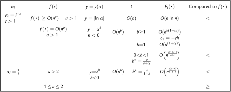
Where b∗ is the optimal value of b.

Assume that

is the goal estimation function under the nondeterministic model with additional computation

. In order for

, if

, then

(constant) and the corresponding distribution function

has to be arbitrarily small. This is equivalent to the goal falling into a certain element with probability one when the additional computation

gradually increases. In statistical inference, it is known that so long as the sample size (or the stopping variable in the Wald sequential probabilistic ratio test) gradually increases the goal can always be detected within a certain element with probability one. Therefore, if regarding the sample size as the additional amount of computation, there exist several statistical inference methods which have the relation

, where the meaning of

is the same as that of the

in the formula

. Then, from Proposition 2.5, it shows that if a proper statistical inference method is applied to multi-granular computing methods, the order of complexity

can reach

regardless of the form of the original complexity f(X).

Tree search is a typical example of multi-granular computing as mentioned in Chapter 1, where

and

, m is the branching factor of the tree. It is expected that tree search will benefit from introducing statistical inference methods to search. More details will be presented in Chapter 6.

2.2.4. Successive Operation in Multi-Granular Computing

From the probabilistic model, it shows that some elements in a certain granular level which contain the goal can only be found with certain probability. It implies that the elements we have already found might not contain any goal. Thus, the mistakes should be corrected as soon as they are discovered. By tracing back, we can go back to some coarse granular level and begin a new round of computation. In our terminology, it is called successive operation. In Chapter 6, we'll show that under certain conditions, by successive operation the goal can be found with probability one but the order of complexity does not increase at all.

..................Content has been hidden....................

You can't read the all page of ebook, please click here login for view all page.

Table of Contents for 2.2. The Estimation of Computational Complexity

Create new playlist

Sign In

Sign Up

2.2. The Estimation of Computational Complexity

2.2.1. The Assumptions

Hypothesis A

Definition 2.1

2.2.2. The Estimation of the Complexity Under Deterministic Models

Local Partition Method

Definition 2.2

Case

Proposition 2.1

Example 2.4

Proposition 2.2

case

Proposition 2.3

Global Partition Method

Proposition 2.4

Example 2.5

2.2.3. The Estimation of the Complexity Under Probabilistic Models

Definition 2.3

Example 2.6

Definition 2.4

Proposition 2.5

Proof:

Proposition 2.6

Proof:

Proposition 2.7

Proof:

Proposition 2.8

Proof:

Proposition 2.9

Proof:

Applications

2.2.4. Successive Operation in Multi-Granular Computing

Table of Contents for
2.2. The Estimation of Computational Complexity