Chapter 13. Macroscopic and Compartmental Models

Search in book...
Toggle Font Controls
Create new playlist

Name your new playlist

Playlist description (optional)
Sign In

Email address

Password

Forgot Password?

or

Continue with Facebook

Continue with Google
Sign Up

Full Name

Email address

Confirm Email Address

Password

or

Continue with Facebook

Continue with Google

Chapter 13. Macroscopic and Compartmental Models

Learning Objectives

After completing this chapter, you will be able to:

Define the concept of a backmixed unit and the assumptions involved in it.
Perform steady state and transient analysis of a backmixed unit.
Show that transient analysis is useful to assess the level of mixing in the system.
Couple backmixed units to form a compartmental model for a reactor or for a large-scale system.
Use compartmental models in engineering analysis of complex systems.
Formulate macroscopic models for two-phase systems.

This chapter elaborates on the principles of macroscopic modeling introduced in Chapter 3 and shows additional applications. As described earlier, in macroscopic analysis, the control volume is sufficiently large; hence the information from the microscale is lost and simple empirical laws or assumptions are needed to “close” the problem. The empirical method of transport coefficients for mass transfer problems is commonly used for closure for purely mass transfer applications. Likewise some assumptions on the mixing pattern in the control volume is needed in conjunction with macroscopic mass balance analysis for reacting systems. This is because the average rate of reaction is needed. But this is an integral of the local values and the local values are unknown in the context of macroscopic balances. We will look at some models to capture the mixing in a macroscopic volume.

One commonly used assumption is that the entire system is well-mixed and at uniform concentration. Such a model was described in Section 3.6 and is widely used as a benchmark in reactor and separation process design. For given equipment it may be therefore important to know to what extent this backmixing assumption is valid. This can be ascertained by a transient analysis and we show how this is useful.

If the system is discovered to be not completely backmixed, then a common modeling approach is to split the reactor into subunits connected in series or in parallel. Such a model is called the compartment model or the tanks or cells in series/parallel model. Each compartment is usually modeled as a completely mixed unit. We show how tracer studies are useful to see how many tanks in series should be used.

The compartmental model approach is also useful for modeling larger scale systems. These type of models find application, for instance, in biomedical engineering (e.g., drug distribution in a complex system such as the human body) and in environmental engineering. Here the complex system is viewed as interconnected macroscopic models consisting of several subunits or compartments. The modeling of such systems is therefore a basic extension of macroscopic analysis. They usually require additional inter-compartmental exchange parameters. We will study some illustrative problems and cite some key references on this. Computations of compartmental systems are also illustrated using MATLAB using a simple two-compartment model as an example.

Macroscopic models are widely used for two phase systems, for example, mixer-settler for liquid–liquid extraction. Each phase is modeled as separate compartments and the mass exchange between the two phases is included as the interaction term connecting the two phases. One simplification is the equilibrium stage model, which is often used in separation processes as a first level of analysis. The key assumption in this model is that the exit streams are assumed to be in equilibrium. Mass conservation together with phase equilibrium models are sufficient to predict the level of separation that can be achieved in the system; mass transfer effects are not included at the first level of modeling. An efficiency parameter is introduced at the second level and this parameter can be calculated if the mixing pattern and mass transfer parameters are known in the contactor. The mixing pattern is often modeled using the tanks in series approach. This approach is also used to simulate many similar fluid–fluid contactors such as bubble columns, rotating disc extraction equipment, and so on; the conceptual framework for this approach is explained.

13.1 Stirred Reactor: The Backmixing Assumption

The starting point in macroscopic modeling is the species conservation equation shown in Chapter 3; it is repeated here for ease of reference:

\begin{matrix} {\dot{M}}_{A, i} - {\dot{M}}_{A, e} - {\dot{M}}_{A, W} + V 〈 R_{A} 〉 = \frac{d}{dt} (M_{A}) & (13.1) \end{matrix}

$\begin{matrix} {\dot{M}}_{A, i} - {\dot{M}}_{A, e} - {\dot{M}}_{A, W} + V 〈 R_{A} 〉 = \frac{d}{dt} (M_{A}) & (13.1) \end{matrix}$

This was applied to a continuous flow reactor in Section 3.6. In this section we revisit this briefly and follow it up by providing more information on the tracer experiments discussed in Section 3.7.

In order to close the reaction term, the backmixing assumption is used at the first level of modeling:

Backmixed assumption: < C_A >= C_A,e

Note that this alone is not sufficient to close < R_A > for nonlinear kinetics. For example for a second-order reaction we have

- < R_{A} > = \frac{1}{V} \int_{V} k_{2} C_{A}^{2} dV

$- < R_{A} > = \frac{1}{V} \int_{V} k_{2} C_{A}^{2} dV$

The right-hand side is the average of $C_{A}^{2}$ $C_{A}^{2}$ , denoted as $〈 C_{A}^{2} 〉$ $〈 C_{A}^{2} 〉$ . This need not be the same as the square of average, that is, (<C_A>)². The two will be equal only if there is no variance in the average concentration at every point in the system. The fluid elements have to be mixed on the microscale for this to happen. Hence an additional assumption that the system is micromixed is also used. In particular, this is true only if the fluid elements are mixed at the molecular level, but it is often used as an approximation. It holds unless the reaction time scale is very small compared to the time scale for mixing. The model can then be closed to this level of approximation.

Performance equations for simple power law kinetics are useful in this context and Equations 3.23 and 3.26 from Chapter 3 apply for a first-order and second-order reaction, respectively.

Fractional order kinetics are often encountered and some caution is needed when the model is used for this purpose. For example, for a zero-order reaction, the exit concentration can become negative numerically, but this not possible based on physical considerations. This sets an upper limit on the Damkohler number, which is defined as follows for a zero-order reaction:

\begin{matrix} Da = \frac{V k_{0}}{Q C_{A, i}} & (13.2) \end{matrix}

$\begin{matrix} Da = \frac{V k_{0}}{Q C_{A, i}} & (13.2) \end{matrix}$

The exit concentration can be obtained by solving the mass balance equation and is given as

c_A,e = 1 – Da

If Da = 1 then the exit concentration becomes zero and is set to zero for any Da value greater than one since the exit concentration cannot be negative. A numerical or analytical solution will generate unrealistic negative values for the concentration in this range. Hence caution has to be exercised while interpreting numerical results.

For more complex kinetics, a numerical solution is used. For multiple reactions, the balance equations are written for each species, A, B, C, and so on, and the resulting set of algebraic equations can be solved numerically. The MATLAB solver FSOLVE is useful for this purpose.

The assumption of backmixing closure can be tested by transient response analysis. The next section shows how this is done; it is a continuation of the information provided in Section 3.7. It may be useful to review that section before proceeding further.

13.2 Transient Balance: Tracer Studies

The extent of backmixing can be characterized by tracer studies, also known as stimulus-response studies. The stimulus represents a change in the inlet conditions and the change in concentration in the outlet as a function of time is measured and represents the response curve to the system. The exit response predicted from a theoretical model is then matched with the experimental data to test some of the model assumptions, for example, whether the well-mixed assumption holds or not.

The starting point for analysis of any tracer study is the transient species balance equation. The appropriate representation for a macroscopic volume follows from Equation 13.1 with appropriate simplifications:

V \frac{d 〈 C_{A} 〉}{dt} = Q C_{A, i} - Q C_{A, e}

$V \frac{d 〈 C_{A} 〉}{dt} = Q C_{A, i} - Q C_{A, e}$

If the system is assumed to be backmixed, then 〈C_A〉 = C_A,e and the model is represented as

\begin{matrix} V \frac{d C_{A, e}}{dt} = Q C_{A, i} - Q C_{A, e} & (13.3) \end{matrix}

$\begin{matrix} V \frac{d C_{A, e}}{dt} = Q C_{A, i} - Q C_{A, e} & (13.3) \end{matrix}$

Two types of tracer injection are common: step injection and pulse or bolus injection. The outlet response for these two cases are presented in the following.

13.2.1 Step Input

A step tracer refers to a case where a feed stream is replaced by a stream containing a tracer at time zero. The initial condition for a step tracer is that at t = 0, < C_A >= 0, that is, there is no tracer in tank to start. Hence C_A,e(t = 0) = 0. The inlet concentration is < C_A >= C_A,i for all t > 0. The solution to Equation 13.3 is then

C_{A, e} = C_{A, i} [1 - exp (- t Q / V)]

$C_{A, e} = C_{A, i} [1 - exp (- t Q / V)]$

This equation is normally written in dimensionless form:

\begin{matrix} c_{A, e} = 1 - exp (- t *) & (13.4) \end{matrix}

$\begin{matrix} c_{A, e} = 1 - exp (- t *) & (13.4) \end{matrix}$

where c_A is scaled with inlet concentration and t* is a dimensionless time defined as t* = tQ/V. This is the ratio of the actual time to the mean residence time in the reactor.

The analysis indicates that the tracer concentration should follow an exponential rise in concentration starting at zero and ending at one. If the experimental data indicates such a pattern then we can treat the system as a well-mixed reactor. Analysis of the tracer data for systems that are not well-mixed is treated in Section 13.2.4.

13.2.2 Pulse or Bolus Input

A pulse or bolus tracer refers to a mode where a quantity of tracer is introduced all at once in a very short duration at time zero. No tracer is injected after this. This section looks at the exit response of the tracer for this case.

The inlet concentration now is C_A,i = 0 since we are dealing with t > 0, that is, after the bolus injection. Hence Equation 13.3, the starting mass balance equation, reduces to

V \frac{d C_{A, e}}{dt} = - Q C_{A, e}

$V \frac{d C_{A, e}}{dt} = - Q C_{A, e}$

The solution for this differential equation is

C_A,e = C₀ exp(–Qt/V) = C₀ exp(–t*)

where C₀ is the integration constant, which has the physical meaning of the initial concentration in the tank at t = 0⁺, that is, immediately after the tracer injection. The initial concentration is not known a priori and depends on the quantity of the tracer injected at time zero; it needs an overall mass balance of A for the total duration of the experiment. Let the quantity of tracer injected be $M$ $M$ . The amount of tracer leaving the system over an interval of time Δt is QC_A,e Δt. The total tracer leaving the system is the integral of this from time zero to infinity. By an overall mass balance for A the total tracer leaving the system must be also equal to the quantity of tracer injected, represented as $M$ $M$ .

Hence

M = \int_{0}^{\infty} Q C_{A, e} dt = \int_{0}^{\infty} Q C_{0} exp (- Qt / V) dt

$M = \int_{0}^{\infty} Q C_{A, e} dt = \int_{0}^{\infty} Q C_{0} exp (- Qt / V) dt$

Performing the integration and rearranging we have $C_{0} = M / V$ $C_{0} = M / V$ , which is known as the tracer strength.

Hence the response to a bolus injection is

C_{A, e} = (M / V) exp (- tQ / V)

$C_{A, e} = (M / V) exp (- tQ / V)$

The bolus injection response is therefore an exponentially decreasing function of time and can be expressed in dimensionless form as

\begin{matrix} c_{A, e} = exp (- t *) & (13.5) \end{matrix}

$\begin{matrix} c_{A, e} = exp (- t *) & (13.5) \end{matrix}$

where c_Ae is equal to C_A,e/(M/V). The response curve for a backmixed reactor for a pulse input is shown in Figure 13.1. Here the response is also shown if the system is in plug flow and for an in between case.

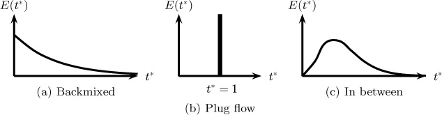
Graphical representation shows the response curve to a pulse tracer.

Figure 13.1 Response curve to a pulse tracer for (a) a system that is completely mixed, (b) a plug flow with the same mean residence time, and (c) a case in between the plug and backmixed cases. Note E(t*) is the dimensionless exit concentration c_A,e.

For the plug flow case in Figure 13.1b, the tracer moves as a plug in the axial direction without any mixing in the flow direction; all the tracer appears at the exit at the same time, equal to the mean residence time. All the fluid in the exit stream has spent the same amount of time in the reactor, equal to the mean residence time.

The response curve for a case where the reactor mixing does not belong to either of the two ideal cases of plug flow and backmixed flow is presented in Figure 13.1c. It should be noted here that the curve shown with a single peak in 13.1c and a spread around a mean value is only applicable to reactors with no severe maldistribution. Such reactors are often termed non-ideal but well behaved. More complex flow patterns such as severe bypassing or large recirculation will show tracer response with multiple peaks. Similarly reactors with large dead volume with poor exchange between active and dead zones (see Figure 3.10) will show a long tail in the tracer response. These cases are sometimes referred to as non-ideal ill-behaved cases.

13.2.3 Age Distribution Functions

In general, the response curves are a measure of time spent by Lagrangian fluid elements in the system; these are characterized by age distribution functions presented in the following subsections. Age means the length of time a fluid has been in the vessel from a Lagrangian perspective. Three age distribution functions are commonly used, as discussed in the following paragraphs.

E-Curve

The dimensionless version of the pulse response is called the E-curve, the exit age distribution curve. The expression for a backmixed reactor follows from Equation 13.5:

E (t *) = exp (- t *) = exp (- tQ / V)

$E (t *) = exp (- t *) = exp (- tQ / V)$

The physical meaning is that E(t*)dt* represents the fraction of the tracer in the exit stream that has spent time between t* and t* + dt*. It represents the fraction of the exit stream that has an age in this interval.

Note that

E(t*)dt* = E(t)dt

Here E(t)dt is the fraction of the tracer in the exit stream that has an age between t and t + dt. This E-curve (in dimensional units) for a backmixed reactor is

\begin{matrix} E (t) = \frac{Q}{V} exp (- t \frac{Q}{V}) = \frac{1}{\bar{t}} exp (- t / \bar{t}) & (13.6) \end{matrix}

$\begin{matrix} E (t) = \frac{Q}{V} exp (- t \frac{Q}{V}) = \frac{1}{\bar{t}} exp (- t / \bar{t}) & (13.6) \end{matrix}$

Here the $\bar{t}$ $\bar{t}$ is the mean residence time, defined as V/Q.

F-Curve

Another age distribution function is the F-curve, F (t). This represents the fraction of the exit stream, which has an age from 0 to t. From the definition it can be shown that the F-curve is the integral of the E-curve and the E-curve is the derivative of the F-curve:

F (t) = \int_{0}^{t} E (t) dt

$F (t) = \int_{0}^{t} E (t) dt$

and

E (t) = \frac{dF}{dt}

$E (t) = \frac{dF}{dt}$

I-Curve

Another age distribution function is the I-curve, I(t), which is called the internal age distribution. I(t)dt represents the fraction of the fluid inside the reactor, which has an age in the range of t and t + dt. The relation between the E-curve and the I-curve follows from the consideration of a fluid of age t either leaving or staying inside the reactor:

I (t) = \frac{Q}{V} [1 - \int_{0}^{t} E (t) dt]

$I (t) = \frac{Q}{V} [1 - \int_{0}^{t} E (t) dt]$

Hence

E (t) = - \frac{V}{Q} \frac{dI (t)}{dt}

$E (t) = - \frac{V}{Q} \frac{dI (t)}{dt}$

13.2.4 Tracer Response for Tanks in Series Model

The previous section showed how the tracer response is useful to identify if the reactor or the process equipment is well mixed. If these experiments show that the system is not well mixed, a model for the reactor needs to be developed. One such model is formulated by assuming that the system is made up of a number of tanks or compartments connected in series. The resulting model is called the tanks in series model and is commonly used in chemical reactor analysis and environmental modeling applications. See Figure 3.9 for an illustration of a vessel modeled as two tanks in series. This approach is also useful for multiphase systems as shown in Section 13.10. In this section we derive an expression for the exit response of such a model.

The system is analyzed by writing the mass balance equations sequentially for each tank with the output from tank 1 serving as the input to tank 2, and so forth. For each tank the transient equation of the type given by Equation 13.3 applies:

\begin{matrix} V_{t} \frac{d C_{A, n}}{dt} = Q (C_{A, n - 1} - C_{A, n}) & (13.7) \end{matrix}

$\begin{matrix} V_{t} \frac{d C_{A, n}}{dt} = Q (C_{A, n - 1} - C_{A, n}) & (13.7) \end{matrix}$

where V_t is the volume of each tank; in dimensionless form we have

\frac{{dc}_{A, n}}{d t *} = c_{A, n - 1} - c_{A, n}

$\frac{{dc}_{A, n}}{d t *} = c_{A, n - 1} - c_{A, n}$

where the concentration is scaled by the tracer strength, assuming all tracer is dispersed in tank 1, and thereby using, $M / (V_{t})$ $M / (V_{t})$ as the concentration scale.

The time is scaled as t* = tQ/V_t, that is, for each tank and not that for the overall reactor. At the end of this section we will correct it to base it on the residence time in the whole tank, where t*, defined as tQ/V, will be used.

A solution to the response curve can be done progressively starting from tank 1 and progressing to tank N. For tank 1 the solution is the same as that for a single tank given earlier (Equation 13.5) with time scaled by the volume of tank 1:

c_A,₁ = exp(–t*)

Hence the equation for tank 2 is

\frac{{d c}_{A, 2}}{d t *} = c_{A, 1} - c_{A, 2}

$\frac{{d c}_{A, 2}}{d t *} = c_{A, 1} - c_{A, 2}$

Substituting the exit from tank 1 as the input to tank 2 we obtain

\frac{{d c}_{A, 2}}{d t *} + c_{A, 2} = exp (- t *)

$\frac{{d c}_{A, 2}}{d t *} + c_{A, 2} = exp (- t *)$

A solution can be obtained using the integrating factor exp(t*). The solution satisfying the initial concentration of zero in tank 2 is

c_A,₂ = t* exp(–t*)

This becomes the input to tank 3 and the differential equation for this tank is

\frac{{d c}_{A, 3}}{d t *} + c_{A, 3} = t * exp (- t *)

$\frac{{d c}_{A, 3}}{d t *} + c_{A, 3} = t * exp (- t *)$

The integration can be continued to give

c_{A, 3} = \frac{{(t *)}^{2}}{2} exp (- t *)

$c_{A, 3} = \frac{{(t *)}^{2}}{2} exp (- t *)$

The result can be generalized to N tanks by inspection:

c_{A, N} = \frac{{(t *)}^{(N - 1)}}{(N - 1)!} exp (- t *)

$c_{A, N} = \frac{{(t *)}^{(N - 1)}}{(N - 1)!} exp (- t *)$

Note that the concentration was scaled by $M / V_{t}$ $M / V_{t}$ . We need to scale it by M/V, the tracer strength based on the reactor volume. Hence we need to multiply the above equation by N to get the new scaled concentration, which is given by

c_{A, N} = N \frac{{(t *)}^{N - 1}}{(N - 1)!} exp (- t *)

$c_{A, N} = N \frac{{(t *)}^{N - 1}}{(N - 1)!} exp (- t *)$

Further, the results are to be expressed in terms of the overall residence time in the reactor, denoted here as t*, which is equal to V_total/Q. Thus t* is replaced by Nt* and the final result for the response of N tanks in series to a pulse of bolus tracer is

\begin{matrix} c_{A, N} = \frac{N^{N}}{(N - 1)!} {(t *)}^{N - 1} exp (- N t *) & (13.8) \end{matrix}

$\begin{matrix} c_{A, N} = \frac{N^{N}}{(N - 1)!} {(t *)}^{N - 1} exp (- N t *) & (13.8) \end{matrix}$

Note that here t* = tQ/V.

The dimensionless time at which the maximum concentration is obtained is obtained by equating the derivative of the above expression with respect to t* equal to zero. The result that this occurs at a dimensionless time of (N – 1)/N is easily verified. Substituting this value of t* in the exit concentration, the maximum value of the exit concentration is obtained as

c_{A,} max = \frac{N (N - 1)^{N - 1}}{(N - 1)!} exp [- (N - 1)]

$c_{A,} max = \frac{N (N - 1)^{N - 1}}{(N - 1)!} exp [- (N - 1)]$

An illustrative response to a system modeled as two and four tanks in series is shown in Figure 13.2 and is compared to a response if the whole tank is assumed to be a single well-mixed tank.

Graphical illustration shows the comparison of a system modeled as two and four tanks in series and a single well-mixed tank.

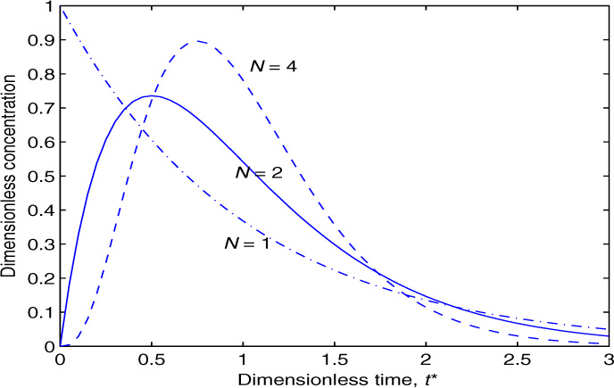
Figure 13.2 Transient concentration profiles in response to a bolus input. Three cases are shown: system modeled as one backmixed tank, system modeled as two tanks in series, four tanks in series.

In summary, the tracer studies are a good way to ascertain the degree of mixing in the system and modify the backmixed assumption as needed. If the system is modeled by tanks in series, then the number of tanks needed to represent the system can be obtained by matching the experimental data with the model values given above. This method is called time domain fitting. An alternative method is moment analysis, which is discussed in the following section.

13.3 Moment Analysis of Tracer Data

An important data analysis tool for the interpretation of the tracer experiments is the method of moments where the expressions for the first and second moments are derived and used to fit the parameters. Let the outlet response, C_A,e, for a pulse input be measured as a function of time. (Note that this data need not be the actual concentration but could be some measure of it, for example, electrical conductivity of a salt solution, color intensity for a dye tracer, and so on.) Then these curves are normalized by the total area under the tracer response curve:

μ_{0} = \int_{0}^{\infty} C_{A, e} dt

$μ_{0} = \int_{0}^{\infty} C_{A, e} dt$

This is a measure of the tracer strength and should be equal to $M / Q$ $M / Q$ since all the injected tracer has to appear in the exit stream sooner or later. The comparison of the experimental μ₀ and the amount of tracer injected also provides a check on the mass balance as well. The μ₀ is also called the zeroth moment.

All concentration data can then be scaled by dividing by μ₀, which provides the response in terms of the dimensionless concentration, c_A,e verus t. The first moment with units of time is defined as

μ_{1} = \int_{0}^{\infty} {t c}_{A, e} dt

$μ_{1} = \int_{0}^{\infty} {t c}_{A, e} dt$

This is a measure of the mean passage time, that is, the time when most of the tracer appears in the exit. This will be equal to V/Q for any closed vessel, that is, a vessel with no back-diffusion or back-flow at the flow boundaries.

The second moment with units of time² is defined as

μ_{2} = \int_{0}^{\infty} t^{2} c_{A, e} d t

$μ_{2} = \int_{0}^{\infty} t^{2} c_{A, e} d t$

A related quantity is the variance σ² (s²), defined as

σ^{2} = μ_{2 -} μ_{1}^{2}

$σ^{2} = μ_{2 -} μ_{1}^{2}$

This is a measure of the spread of the tracer around the mean passage time.

Higher order moments can also be defined, for example the nth moment is

μ_{n} = \int_{0}^{\infty} t^{n} c_{A, e} d t

$μ_{n} = \int_{0}^{\infty} t^{n} c_{A, e} d t$

However these are not commonly used in data analysis since these higher order integrals cannot be accurately calculated from the measured data.

In the moments analysis method, the measured values of the moments are compared to theoretical values and the parameters of the model are fitted. Usually the second central moment or the variance is compared. The calculation of theoretical values is discussed next.

13.3.1 Moments from Laplace Transform of Response

Moments are related to the response curve in the Laplace domain and the method of deriving the needed expressions is presented in the following.

The Laplace transform of the tracer response is defined as

\begin{matrix} {\bar{c}}_{A, e} (s) = \int_{0}^{\infty} exp (- s t) c_{A, e} (t) d t & (13.9) \end{matrix}

$\begin{matrix} {\bar{c}}_{A, e} (s) = \int_{0}^{\infty} exp (- s t) c_{A, e} (t) d t & (13.9) \end{matrix}$

where s is the transform parameter. Note that the integration is with respect to t for various values of the parameter s.

If the exponential function is expanded the integral on the right-hand side of Equation 13.9 can be written as

{\bar{c}}_{A, e} (s) = \int_{0}^{\infty} (1 - st + \frac{s^{2} t^{2}}{2} + \dots) c_{A, e} d t

${\bar{c}}_{A, e} (s) = \int_{0}^{\infty} (1 - st + \frac{s^{2} t^{2}}{2} + \dots) c_{A, e} d t$

If we expand the left-hand side of Equation 13.9 in a Taylor series, we have

{\bar{c}}_{A, e} (s) = {\bar{c}}_{A, e} (s = 0) + s {(\frac{{d \bar{c}}_{A, e}}{ds})}_{s = 0} + \frac{s^{2}}{2} {(\frac{d^{2} {\bar{c}}_{A, e}}{d^{2} s})}_{s = 0} + \dots

${\bar{c}}_{A, e} (s) = {\bar{c}}_{A, e} (s = 0) + s {(\frac{{d \bar{c}}_{A, e}}{ds})}_{s = 0} + \frac{s^{2}}{2} {(\frac{d^{2} {\bar{c}}_{A, e}}{d^{2} s})}_{s = 0} + \dots$

Equating terms with the same power of s on either side the following relations are obtained. For s = 0 we get

{\bar{c}}_{A, e} (s = 0) = \int_{0}^{\infty} {\bar{c}}_{A, e} d t = 1

${\bar{c}}_{A, e} (s = 0) = \int_{0}^{\infty} {\bar{c}}_{A, e} d t = 1$

which is the dimensionless tracer strength.

The (scaled) first moment is then related to the first derivative of the response in the Laplace domain:

μ_{1} = \int_{0}^{\infty} {t c}_{A, e} d t = - {(\frac{{d \bar{c}}_{A, e}}{ds})}_{s = 0}

$μ_{1} = \int_{0}^{\infty} {t c}_{A, e} d t = - {(\frac{{d \bar{c}}_{A, e}}{ds})}_{s = 0}$

The second moment is

μ_{2} = \int_{0}^{\infty} t^{2} c_{A, e} d t = {(\frac{{d^{2} \bar{c}}_{A, e}}{d s^{2}})}_{s = 0}

$μ_{2} = \int_{0}^{\infty} t^{2} c_{A, e} d t = {(\frac{{d^{2} \bar{c}}_{A, e}}{d s^{2}})}_{s = 0}$

Expressions for additional moments can be derived if needed. In general

μ_{n} = \int_{0}^{\infty} t^{n} c_{A, e} d t = {(- 1)}^{n} {(\frac{{d^{n} \bar{c}}_{A, e}}{d s^{n}})}_{s = 0}

$μ_{n} = \int_{0}^{\infty} t^{n} c_{A, e} d t = {(- 1)}^{n} {(\frac{{d^{n} \bar{c}}_{A, e}}{d s^{n}})}_{s = 0}$

Thus all the moments can be generated from the solution in the Laplace domain. An illustration of derivation of the Laplace transform and the expression for the second moment is shown in Example 13.1.

Example 13.1 Moments for N Tanks in Series

Derive an expression for the response to N tanks in series in the Laplace domain. From the solution derive expressions for the first and second moment and the variance of the response curve.

Solution

For each tank the transient equation of the type given by Equation 13.7 applies:

V_{t} \frac{d C_{A, n}}{dt} = Q (C_{A, n - 1} - C_{A, n})

$V_{t} \frac{d C_{A, n}}{dt} = Q (C_{A, n - 1} - C_{A, n})$

V_t is the volume of each tank. Since V_t = V/N, this can be written as

\frac{V}{QN} \frac{d c_{A, n}}{dt} = (c_{A, n - 1} - c_{A, n})

$\frac{V}{QN} \frac{d c_{A, n}}{dt} = (c_{A, n - 1} - c_{A, n})$

Here the concentration has been normalized by dividing C_A by the tracer strength for the pulse tracer.

Taking the Laplace transform of the previous equation we get

\frac{V}{QN} s {\bar{c}}_{A, n} = {\bar{c}}_{A, n - 1} - {\bar{c}}_{A, n}

$\frac{V}{QN} s {\bar{c}}_{A, n} = {\bar{c}}_{A, n - 1} - {\bar{c}}_{A, n}$

Note that the initial concentration is taken as zero here. Rearranging, we get the response of the nth tank in terms of the response from the n – 1 tank:

{\bar{c}}_{A, n} = \frac{{\bar{c}}_{A, n - 1}}{(1 + sV / QN)}

${\bar{c}}_{A, n} = \frac{{\bar{c}}_{A, n - 1}}{(1 + sV / QN)}$

Starting from tank 1 we can get the response of tank 2 and continuing we get the response for N tanks as

{\bar{c}}_{A, e} = \frac{{\bar{c}}_{A, i}}{(1 + sV / QN)^{N}}

${\bar{c}}_{A, e} = \frac{{\bar{c}}_{A, i}}{(1 + sV / QN)^{N}}$

where ${\bar{c}}_{A, i}$ ${\bar{c}}_{A, i}$ is the Laplace transform of the inlet concentration. For a pulse response ${\bar{c}}_{A, i} = 1$ ${\bar{c}}_{A, i} = 1$ and hence the response curve in the Laplace domain is

{\bar{c}}_{A, e} = \frac{1}{(1 + sV / QN)^{N}}

${\bar{c}}_{A, e} = \frac{1}{(1 + sV / QN)^{N}}$

Taking the derivative and setting s = 0 we find μ₁ = V/Q, which is equal to the mean residence time $\bar{t}$ $\bar{t}$ .

Similarly μ₂ is found by taking the second derivative and you should verify that

μ_{2} = [(N + 1) / N] (V / Q)^{2}

$μ_{2} = [(N + 1) / N] (V / Q)^{2}$

The variance, σ², is calculated as $μ_{2} - μ_{1}^{2}$ $μ_{2} - μ_{1}^{2}$ . This gives us

σ^{2} = \frac{1}{N} (\frac{V}{Q})^{2}

$σ^{2} = \frac{1}{N} (\frac{V}{Q})^{2}$

This has units of s². A dimensionless variance is often defined and used as follows:

\begin{matrix} \begin{matrix} {(σ *)}^{2} = \frac{σ^{2}}{{\bar{t}}^{2}} = \frac{1}{N} \end{matrix} & (13.10) \end{matrix}

$\begin{matrix} \begin{matrix} {(σ *)}^{2} = \frac{σ^{2}}{{\bar{t}}^{2}} = \frac{1}{N} \end{matrix} & (13.10) \end{matrix}$

\bar{t}

$\bar{t}$ is the mean passage time equal to V/Q. This equation is a classical result for N tanks in series and can be matched with the experimental variance to find the representation of the reactor in the tanks in series model.

It is interesting to note that the response curve in the time domain can be reconstructed within engineering accuracy from the moments using the Laguerre polynomials. The Laplace inversion is not needed when using this method since the inverse transform calculations can in some cases involve lengthy mathematical manipulations. The full discussion is given by Linek and Dudukovic (1982) and further details are not addressed here.

13.4 Tanks in Series Models: Reactor Performance

In this section, we calculate the reactor performance when the reactor is modeled as N tanks connected in series. For a first-order reaction, the species mass balance for any compartment n leads to

Q(C_A,n–1 – C_A,n) = V_tk₁C_A,n

where V_t is the volume of each tank. Since V_t = V/N, this can be written as

\begin{matrix} c_{A, n - 1} - c_{A, n} = \frac{V k_{1}}{QN} c_{A, n} = \frac{Da}{N} c_{A, n} & (13.11) \end{matrix}

$\begin{matrix} c_{A, n - 1} - c_{A, n} = \frac{V k_{1}}{QN} c_{A, n} = \frac{Da}{N} c_{A, n} & (13.11) \end{matrix}$

The concentration has been normalized by the inlet concentration. The Da parameter is the Damkohler number, based on the volume V of the reactor. Equation 13.11 can be rearranged to:

c_{A, n} = \frac{c_{A, n - 1}}{1 + Da / N}

$c_{A, n} = \frac{c_{A, n - 1}}{1 + Da / N}$

Starting from n = 1, the first compartment and progressing to the Nth compartment we find the exit concentration in the reactor:

\begin{matrix} c_{A, N} = \frac{1}{(1 + Da / N)^{N}} & (13.12) \end{matrix}

$\begin{matrix} c_{A, N} = \frac{1}{(1 + Da / N)^{N}} & (13.12) \end{matrix}$

Nonlinear reactions are solved by writing equations similar to 13.11 and solving the set of the resulting set of N algebraic equations numerically. No new concepts are involved in modeling these but closed-form solutions may not be obtained, unlike the first-order case. Note that Damkohler number is a function of the inlet concentration for nonlinear kinetics, unlike the case of a first-order reaction. Multiple species and multiple reactions are handled by a similar approach.

An assumption involved in this modeling approach is that the fluid is mixed all the way to the micro level. If the fluid is mixed only at a macro level the method discussed in the following section is used. For linear kinetics it does not matter whether the fluid is mixed on a macro or micro level.

13.5 Macrofluid Models

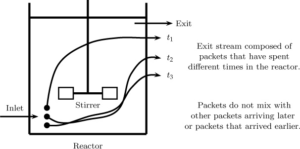
Here we show how the exit age distribution is useful to predict the conversion in a reactor assuming the system is well mixed but only on a macro level. The following assumption is made for this analysis: different elements entering the reactor at different times remain segregated and do not mix with elements that have entered earlier or elements that stay behind for a longer time.

The exit stream is visualized as a mixture of different macrofluid parcels that have spent different amounts of time in the reactor. The situation is illustrated in Figure 13.3.

Diagrammatic illustration of macrofluid models.

Figure 13.3 The macrofluid representation of a reactor: segregation on an age basis.

An element spending time t would have reacted as

\begin{matrix} \frac{d C_{A}}{dt} = R_{A} (C_{A}) & (13.13) \end{matrix}

$\begin{matrix} \frac{d C_{A}}{dt} = R_{A} (C_{A}) & (13.13) \end{matrix}$

The integration provides us a C_A(t) function for any specified form of R_A.

The exit stream is composed of elements of many ages, each spending a time t. The fraction of the exit stream that has spent time t is E(t)dt. Hence the contribution to the exit conversion for the element of age t is C_A(t)E(t)dt. The exit concentration, summing for all ages, is thus

\begin{matrix} \begin{matrix} C_{A, e} = \int_{0}^{\infty} C_{A} (t) E (t) dt \end{matrix} & (13.14) \end{matrix}

$\begin{matrix} \begin{matrix} C_{A, e} = \int_{0}^{\infty} C_{A} (t) E (t) dt \end{matrix} & (13.14) \end{matrix}$

C_A as a function of time is obtained from the solution of Equation 13.13 and results in the same expression as for a batch reactor. It can be shown that the results for macrofluid models and microfluid models are the same for a first-order reaction. An example follows for a second-order reaction for a backmixed reactor.

13.5.1 Second-Order Reaction

For a second-order reaction in a batch reactor we can show that the concentration of a stream that has spent a time t in the reactor is:

c_{A} (t) = \frac{1}{1 + k_{2} C_{A, i} t}

$c_{A} (t) = \frac{1}{1 + k_{2} C_{A, i} t}$

Combining this with the exit age distribution for a backmixed system (Equation 13.6), we obtain

E (t) = \frac{1}{\bar{t}} exp (- t / \bar{t})

$E (t) = \frac{1}{\bar{t}} exp (- t / \bar{t})$

Using these results in Equation 13.14 we get

c_{A, e} = \int_{0}^{\infty} \frac{1}{1 + k_{2} C_{A, i} t} \frac{exp (- t / \bar{t})}{\bar{t}} dt

$c_{A, e} = \int_{0}^{\infty} \frac{1}{1 + k_{2} C_{A, i} t} \frac{exp (- t / \bar{t})}{\bar{t}} dt$

The integral can be evaluated numerically as shown in Listing 13.1. But a closed-form analytical solution can be obtained:

\begin{matrix} c_{A, e} = \frac{C_{A, e}}{C_{A, i}} = \frac{1}{Da} exp (- 1 / Da) Ei (1 / Da) & (13.15) \end{matrix}

$\begin{matrix} c_{A, e} = \frac{C_{A, e}}{C_{A, i}} = \frac{1}{Da} exp (- 1 / Da) Ei (1 / Da) & (13.15) \end{matrix}$

where Ei is an exponential integral, a tabulated mathematical function. This function is readily calculated in MATLAB as expint. Table 3.1 in Chapter 3 showed the results comparing the microfluid and microfluid approach for a second-order reaction; we find that the macromixing conditions provide a lower concentration and therefore a higher conversion.

Table 13.1 Comparison of Micro versus Segregation Model: Results for a Backmixed Reactor for Zero-Order Kinetics

Da	c_A,e, Microfluid	c_A,e, Macrofluid
0.1	0.9	0.9
0.5	0.5	0.5677
1.0	0.0	0.3679
5.0	0.0	0.0937
10.0	0.0	0.0484

13.5.2 Zero-Order Reaction

The concentration change for a zero-order reaction is given as

c_A,e = 1 – k₀t/C_A,i t ≤ C_A,i/k₀

and C_A,e = 0 if t > C_A,i/k₀. Using this together with the expression for E(t) in Equation 13.14, the result for exit conversion can be determined to be

\begin{matrix} c_{A, e} = \frac{C_{Ae}}{C_{A, i}} = 1 - Da + Da exp (- 1 / Da) & (13.16) \end{matrix}

$\begin{matrix} c_{A, e} = \frac{C_{Ae}}{C_{A, i}} = 1 - Da + Da exp (- 1 / Da) & (13.16) \end{matrix}$

where Da is the Damkohler number defined earlier by Equation 13.2. The derivation is left as an exercise problem. The comparison is shown in Table 13.1. The conversion is lower if the fluid is macromixed, a trend opposite to the second-order case.

The previous two examples provide illustrations of the macrofluid model for second-order and zero-order kinetics. For the general case, it is easier to calculate this by writing the small computational snippet presented in Listing 13.1.

Listing 13.1 Macrofluid Model Calculations with MATLAB+CHEBFUN

Click here to view code image

% conversion in a CSTR assuming a macrofluid.
Da = 10.0;
d = [0, 30]; % domain; t_max = 30 used.
t = chebfun('t',d); % x variable
L = chebop(d); % name of operator
L.op = @(c) diff(c,1)+ Da*c.^2; % second order reaction
L.lbc = @(c) [c–1]; % inlet condition
c = L; % batch concentration for time t.
% define exit age curve; CSTR used here
% note t is dimensionless (t/tbar).
E = exp(–t) ; % E–theta curve
% use sum command or quad function to integrate.
c_exit_macro = sum (c.*E)
% analytical solution for comparison (for second order)
c1 = 1/Da * exp(1/Da)* expint (1/Da)

The infinte domain for dimensionless time integration was replaced by 30 as the upper limit. Zero-order reactions need small modifications. Only dimensionless time less than 1/Da contributes to the exit concentration. Hence the domain should be changed to 1/Da.

The result for Da = 10 for a zero-order reaction should be 0.0408 as in Table 13.1 or could be computed from the analytical solution given by Equation 13.16. Note that even when Da = 10, complete conversion is not achieved. Elements exiting earlier have remained nearly unreacted!

13.6 Variance-Based Models for Partial Micromixing

This section may be omitted without loss of continuity.

Here we present some results where the variance in concentration in the reactor is used as an additional variable to predict the effects of deviation from complete micromixing. Such models are developed from a detailed population balance model and details are shown in Froment, Bischoff, and Wilde (2011). The goal of this section is to merely present the key results so that you get an overview of these models. The conceptual basis for the model shown here is useful if you wish to pursue the study and applications of these models further.

The key idea is that the concentration in the reactor can be defined by a probability distribution function f that can then be used to find an average concentration and also its variance. The fraction of the reactor volume having a concentration of C_A in the interval of dC_A is then equal to f(C_A)dC_A. The average concentration is then

〈 c_{A} 〉 = \int_{0}^{C_{A, i}} C_{A} f (C_{A}) d C_{A}

$〈 c_{A} 〉 = \int_{0}^{C_{A, i}} C_{A} f (C_{A}) d C_{A}$

This is the same is the exit concentration C_A,e for a well-mixed system. The variance of the concentration around the mean is defined as

σ_{R}^{2} = \int C_{A}^{2} f (C_{A}) d C_{A} - {[〈 c_{A} 〉]}^{2}

$σ_{R}^{2} = \int C_{A}^{2} f (C_{A}) d C_{A} - {[〈 c_{A} 〉]}^{2}$

The variance is non-zero unless the reactor is perfectly mixed.

The population balance model provides a differential equation for the f function. (A number of closure models are needed including the birth and death rate of the population [concentration] in each interval.) The details are not shown here. Using this the following relations can be derived.

For a first-order reaction the following equation can be derived for the dimensionless variance of the concentration in the reactor:

{σ *}^{2} = \frac{σ_{R}^{2}}{C_{A, e}^{2}} = \frac{D a^{2}}{2 Da + β \bar{t} + 1}

${σ *}^{2} = \frac{σ_{R}^{2}}{C_{A, e}^{2}} = \frac{D a^{2}}{2 Da + β \bar{t} + 1}$

where β is a micromixing parameter that characterizes the level of micromixing in the system, with β of infinity representing perfect micro-mixing. Of course the variance has no effect on the average concentration for a first-order reaction, which is given as 1/(1 + Da) as shown earlier. The estimate of the variance here is mainly useful for experimental verification of mixing effects in the reactor.

For a second-order reaction the average rate of reaction now depends also on the variance and therefore on how close the reactor is to micromixing. For the latter case, the variance is zero and the micromixing model shown in Section 3.6 applies. If the reactor is not completely micromixed then the exit concentration can be given by the following equation:

1 - c_{A, e} = Da c_{A, e}^{2} (1 + {σ *}^{2})

$1 - c_{A, e} = Da c_{A, e}^{2} (1 + {σ *}^{2})$

Hence an additional equation for the variance is derived and solved. This equation for a second-order reaction can be determined to be

(4 {D a c}_{A, e} + β \bar{t} + 1) {σ *}^{2} = {D a c}_{A . e} {({σ *}^{2} + 1)}^{2}

$(4 {D a c}_{A, e} + β \bar{t} + 1) {σ *}^{2} = {D a c}_{A . e} {({σ *}^{2} + 1)}^{2}$

The above two equations are solved simultaneously for a given value of the micromixing parameter, β. An estimate of this micromixing parameter is needed for these calculations. An approximate value of β = 0.5s^–1 is a useful estimate for low viscosity fluids in standard process vessels (Froment et al., 2011). For viscous fluids β is much smaller and deviation from perfect micromixing can become important. Evangelista (1969) suggests that β scales as

β = K {(\frac{ɛ}{L^{2}})}^{1 / 3}

$β = K {(\frac{ɛ}{L^{2}})}^{1 / 3}$

Here ∊ is the power input per mass of the system and L is a characteristic length parameter of the vessel.

13.7 Compartmental Models

Complex systems such as the human body or the environment are often modeled using compartmental models. Conceptually this is similar to the tanks in series model discussed earlier; the only difference is the interconnectivity of compartments can be quite complex. A complex system is therefore treated as a network of interconnected compartments and macroscopic balances (usually) are applied to each compartment. Thus a complete system is viewed as a network of perfectly mixed cells connected in some suitable manner. The compartments can exchange mass with each other. The schematic basis of the compartment model is shown in Figure 13.4.

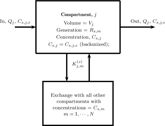
Diagrammatic representation of compartmental model.

Figure 13.4 Schematic of a compartmental model showing the mass balance for compartment j.

The mass balance for each species takes the following form:

\begin{matrix} V_{j} \frac{d (C_{s, j})}{d t} = Q_{j, i} C_{s, j, i} - Q_{j, e} C_{s, j} + \sum_{m = 1}^{N T} K_{m, j}^{(s)} (C_{s, m} - C_{s, j}) + V_{j} R_{s, j} & (13.17) \end{matrix}

$\begin{matrix} V_{j} \frac{d (C_{s, j})}{d t} = Q_{j, i} C_{s, j, i} - Q_{j, e} C_{s, j} + \sum_{m = 1}^{N T} K_{m, j}^{(s)} (C_{s, m} - C_{s, j}) + V_{j} R_{s, j} & (13.17) \end{matrix}$

The notations are pertinent to those shown in Figure 13.4. Here the subscript s refers to species, and j refers to a tank. Total number of tanks is NT; they are all assumed to be interconnected with each tank exchanging mass with other tanks. The summation term on the right-hand side accounts for this interaction. The rate of exchange is K_m,j, which represents the moles or mass of species under consideration being transferred from compartment m to compartment j. Various species (index s) may have different exchange coefficients.

Hence K_m,j is tagged as $K_{m, j}^{(s)}$ $K_{m, j}^{(s)}$ .

Examples of compartmental models are widespread in biomedical systems, pharmacokinetic analysis, environmental systems, and chemical reactor modeling. We now discuss some computational aspects of the compartmental model with one application. This problem also illustrates the application of the linear algebra technique to solve differential equations. Additional problems at the end of the chapter provide more information.

13.7.1 Matrix Representation

The following assumptions are commonly made to simplify the computation of the model given by Equation 13.17:

Mixing assumption: Each compartment is assumed to be well mixed and the concentration in the compartment is the same as the exit concentration of that compartment.
Reaction kinetics: The reaction is assumed to be first order.

These assumptions reduce the model equations into a linear form and the compartmental model can be generalized using matrix-vector representation:

\begin{matrix} \frac{dy}{dt} = \tilde{A} y + R & (13.18) \end{matrix}

$\begin{matrix} \frac{dy}{dt} = \tilde{A} y + R & (13.18) \end{matrix}$

Here y is the solution vector consisting of the concentration values in each compartment. You should work out what the coefficient matrix A and the vector R are for the case represented by Equation 13.17. We discuss the solution here for the case where A and R are constants. The formal solution to such problems can be represented using the concepts of eigenvectors and eigenvalues of a matrix and the concept of the matrix exponential. Recall that if y is a scalar variable then the solution to Equation 13.18 is

y = B₁ exp(At) – R/A

where B₁ is an integration constant. The solution consists of two parts: a homogeneous solution and a particular solution.

The constant of integration B₁ can be evaluated from the initial condition: if y(t = 0) = y₀ then the solution can be written as

y = (y₀ + R/A) exp(At) – R/A

The solution for multiple systems of initial value problems (IVP) is represented in exactly same manner as that for a single equation: the solution is

\begin{matrix} y = exp (\tilde{A} t) [y_{0} + {\tilde{A}}^{- 1} R] - {\tilde{A}}^{- 1} R & (13.19) \end{matrix}

$\begin{matrix} y = exp (\tilde{A} t) [y_{0} + {\tilde{A}}^{- 1} R] - {\tilde{A}}^{- 1} R & (13.19) \end{matrix}$

Here exp is the exponential of a matrix, which can be readily computed using the function expm in MATLAB. y₀ is the vector of initial values. Using this format the MATLAB implementation of the compartmental model is relatively simple and useful.

Note that the exponential of a matrix is defined similarly to an exponential function. This is simply a power series in matrix form and the formal representation is

exp (\tilde{A}) = \tilde{I} + \tilde{A} + \frac{{\tilde{A}}^{2}}{2!} + \frac{{\tilde{A}}^{3}}{3!} + \dots

$exp (\tilde{A}) = \tilde{I} + \tilde{A} + \frac{{\tilde{A}}^{2}}{2!} + \frac{{\tilde{A}}^{3}}{3!} + \dots$

However, the numerical implementation uses a method based on the Pade approximations and avoids computing all the powers of the matrix Ã.

The use of MAPLE provides the exponential matrix in a symbolic form rather than the numerical values at a given instant of time. Sample code segments are given by White and Subramanian (2010). Example 13.2 shows an illustrative application.

Example 13.2 A two-compartment model for pharmacokinetic analysis

Set up the model equations for the two-compartment model shown in Figure 1.12 (Chapter 1) for analysis of drug distribution in a body. Solve for the illustrative parameters. Study the effect of the exchange parameter K_ex on the response of the system.

Solution

Apply Equation 13.17 for each compartment. The following equations should result.

For compartment 1, the blood compartment:

\begin{matrix} V_{1} \frac{d C_{1}}{dt} = Q_{1, i n} C_{0} - Q_{1, o u t} C_{1} + K_{ex} (C_{2} - C_{1}) - V_{1} k_{1} C_{1} & (13.20) \end{matrix}

$\begin{matrix} V_{1} \frac{d C_{1}}{dt} = Q_{1, i n} C_{0} - Q_{1, o u t} C_{1} + K_{ex} (C_{2} - C_{1}) - V_{1} k_{1} C_{1} & (13.20) \end{matrix}$

For compartment 2, the tissue compartment:

\begin{matrix} V_{2} \frac{d C_{2}}{dt} = Q_{2, i n} C_{2, i n} - Q_{2, o u t} C_{2} + K_{ex} (C_{1} - C_{2}) - V_{2} k_{2} C_{2} & (13.21) \end{matrix}

$\begin{matrix} V_{2} \frac{d C_{2}}{dt} = Q_{2, i n} C_{2, i n} - Q_{2, o u t} C_{2} + K_{ex} (C_{1} - C_{2}) - V_{2} k_{2} C_{2} & (13.21) \end{matrix}$

We obtain a system of two differential equations that can be expressed in the compact matrix-vector form shown in Equation 13.18. Also the flow terms Q₁ and Q₂ are set as zero; thereby a simpler model is generated. The y vector is composed of C₁ and C₂. The solution can then be computed directly using the expm function or can also be implemented numerically using ODE45 or ODE15s if the equations are stiff (defined at the end of this section).

An illustrative result is shown in Figure 13.5 for the following parameter values: V₁ = 1, V₂ = 3, k₁ = 0.2, k₂ = 2.0, and K_ex = 5.0 in arbitrary units. The results for K_ex = 50 are shown in Figure 13.6.

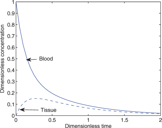
Graphical representation of the transient concentration profiles for a two-compartment model.

Figure 13.5 Transient concentration profiles in response to a bolus input for a two-compartment model.

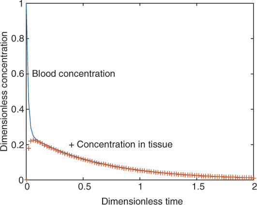
Figure 13.6 Transient concentration profiles in response to a bolus input for a two-compartment model. K_ex = 50.

For the second case, since the exchange parameters are large, we find that there is an initial fast decay where the tracer exchanges mass with the tissue. Both blood and tissue reach the same concentration in a short time. This is followed by metabolism in tissue compartments (which is now in equilibrium with the blood compartment) leading to a slow decay in the system. In some cases it may be difficult to experimentally detect the initial fast decay and exercise problem 8 deals with some of these issues.

13.8 Compartmental Models for Environmental Transport

Compartmental models are widely used in environmental engineering for prediction of the environmental fate of chemicals. The goal of this section is to provide a brief overview on this topic. Some useful references are also provided for readers who wish to pursue this topic further.

The fate of chemicals released into the environment is important in predicting the exposure risk of chemicals. This is dependent on two factors:

Translocation: Will it stay in the same place (e.g., in air) or if not, where will it go?
Transformation: Will its chemical composition be altered by chemical reaction?

Models to predict this information require defining some type of large-scale compartmental model, sometimes referred to as a megascopic model. The environment can be considered to be composed of four broad compartments, that is air, water, soil, and biota (which includes plant and animals) (see Figure 1.14).

The simplest model considers each compartment a lumped system and the macroscopic level compartmental models described in this chapter are then used for each compartment. Such models are useful for evolution at very large scales (e.g., at the global level). More detailed models with greater levels of segmentation and spatial variation in each compartment are best suited for site-specific analysis problems (e.g., locations near a chemical industry). It should be noted that as the model complexity increases, its resolution and the data needed for prediction also increase.

Mackay et al. (1996a, 1996b, 1996c) and Mackay (2001) suggest modeling at three levels (later extended to four levels) and a brief description of these levels together with the data needed at each level is provided in the following subsections to provide a general overview.

13.8.1 Fugacity of Pollutants in Each Compartment

The fugacity is used as basic variable in these models and the fugacity difference between two compartments is used as the driving force in defining the inter-compartmental exchange term. The concentration jump across the interface of each compartment is then automatically accounted for. Fugacity is like a single currency! The concentration and the fugacity in each compartment are related by defining a fugacity capacity factor. Thus

\begin{matrix} C_{A, j} = f_{A, j} Z_{A, j} & (13.22) \end{matrix}

$\begin{matrix} C_{A, j} = f_{A, j} Z_{A, j} & (13.22) \end{matrix}$

Here f_A,j is the fugacity of A in compartment j, C_A,j is its concentration, and Z_A,j is the fugacity capacity factor. The latter will depend on the thermodynamic equilibrium relation for each compartment relative to the air phase and the relations can be calculated as follows.

For air, using the ideal gas law the fugacity is the same as the partial pressure of A and hence Z_A = 1/R_gT.

For water, using Henry’s law, p_A = H_AC_AL, and equating the fugacities at equilibrium conditions, it is easy to show that Z_A = 1/H_A.

For soil, the following relation (again based on equal fugacity of A in soil and air) was suggested:

Z_A(soil) = x_AcK_OCρ_s/H_A

where x_Ac is the mole fraction of organic carbon in the soil, and K_OC is the organic carbon partition coefficient in the soil. This is related to the octanol-water partition coefficient K_OW as 0.41K_OW.

For biota, the following relation (again based on equal fugacity of A in soil and air) was suggested by Paterson (1991):

Z_A(biota) = 0.048K_OW ρ_b/H_A

13.8.2 Level I or Equilibrium Model

A Level I simulation is the equilibrium distribution of a fixed quantity of conserved (i.e., non-reacting) chemical, in a closed environment at equilibrium, with no degrading reactions, no advective processes, and no intermedia transport processes. The medium receiving the emission is unimportant because the chemical is assumed to become instantaneously distributed to an equilibrium condition.

Computations at this level are done using the following approach. The total moles in the system is

\begin{matrix} M_{A} (total) = \sum_{j} V_{j} C_{A j} = f_{A} \sum_{j} V_{j} Z_{A j} & (13.23) \end{matrix}

$\begin{matrix} M_{A} (total) = \sum_{j} V_{j} C_{A j} = f_{A} \sum_{j} V_{j} Z_{A j} & (13.23) \end{matrix}$

Here V_j is the volume of compartment j. $M_{A}$ $M_{A}$ is the total moles of A released into one or more of the compartments. Note that the fugacity term is outside the summation since it is the same in all the compartments. This is an advantage of the fugacity approach where a single currency is being used. Hence fractional distribution of species A in compartment j is equal to

f_{j, A} = \frac{V_{j} Z_{Aj}}{\sum_{j} V_{j} Z_{Aj}}

$f_{j, A} = \frac{V_{j} Z_{Aj}}{\sum_{j} V_{j} Z_{Aj}}$

This provides the translocation information. The data needed are physical-chemical properties to find the fugacity capacity factors and the user-defined compartment volumes and densities.

This model is useful for establishing the general features of a new or existing chemical’s behavior and provides the likely media into which a chemical will tend to partition.

13.8.3 Level II Model: Advection Effects

This model is similar to Level I, but is a steady state model with a constant input rate, rather than a single dose of chemical. There is both advective in-and outflow of chemicals from the unit world. Chemical losses can also occur through degrading reactions. Equilibrium is assumed in each compartment. Equations similar to Equation 13.17 (with no accumulation and no exchange term) are then written for each compartment and solved simultaneously.

In addition to the data required for Level I the following must be input: emission rate in lieu of amount of chemical, advective inflow rates, inflow concentration, and reaction half-lives of the chemical in each medium.

13.8.4 Level III Model: Intermedia Transport Effects

This level does not assume an equilibrium state between the compartments, but only steady state. In addition to the data required for Level II the following must be input: intermedia transfer rates and related parameters such as airside mass transfer coefficient, water-side mass transfer coefficient, rain rate, aerosol deposition, and so on. The program uses conventional expressions and typical parameters for intermedia transfer by processes such as wet deposition from the air, sediment deposition in the water, and soil runoff. If intermedia transfer rates are not known, then a generic version of the model uses a set of pre-assigned transfer rates.

More details can be found in Paterson (1991) and Mackay (2001). Model formulation is very similar to the compartmental models described earlier in this section. The main difference is that fugacity is used as the primary variable rather than the concentration.

A note of caution is useful here. These models cannot be as such validated in the same sense as some other models in mass transfer, for example, a model for simple equipment such as an absorber. Only an order of magnitude fit can be expected, but even with this limitation, the model predictions are very useful for predicting the likely behavior of new chemicals and their environmental impact.

13.8.5 Level IV Model: Transient Effects

This is an extension of the Level III model and the dynamics of emissions and resulting temporal concentration changes are taken into account. This model is complex and is not widely used; Level III is more common. A thesis by Kilic (2008) is illustrative of the use of this model to predict the pollutant levels in rivers.

13.9 Fluid–Fluid Systems

In this section we show modeling concepts for two-phase flows with the assumption that both phases are backmixed. This is the simplest model and leads to algebraic equations that can be readily solved. The discussion is shown for a gas–liquid case but the method is very similar for the liquid–liquid case as well.

13.9.1 Backmixed–Backmixed Model

A schematic description of the model is shown in Figure 13.7.

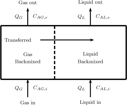
Diagrammatic representation of a two-phase backmixed system.

Figure 13.7 Schematic of a two-phase backmixed–backmixed system showing the control volumes for species mass balance.

Let us consider dilute systems to illustrate the key features of modeling this system. The extension to non-dilute systems is slightly lengthy and generally uses the mole ratio as a variable rather than the mole fraction. But this does not require any new concepts and the dilute system analysis can be extended to these cases.

The dilute system assumption means that the gas molar flow rate and the liquid molar flow rate are nearly constant in the inlet and outlet of the separator. Further a linear equilibrium is assumed and represented in terms of a Henry parameter:

C_AG = H_AC_AL at equilibrium

The gas and liquid phase balances for a dilute system are as follows:

Gas phase balance:

Q_G(C_AG,i – C_AG,e) – K_Ga_glV_C(C_AG,e – H_AC_AL,e) = 0

Liquid phase balance:

Q_L(C_AL,i – C_AL,e) + K_Ga_glV_C(C_AG,e – H_AC_AL,e) = 0

It is more useful to solve these in terms of dimensionless concentrations and dimensionless parameters. The concentration in the gas phase is made dimensionless with respect to the inlet gas concentration. Thus we define

c_{A G, e} = \frac{C_{AG . e}}{C_{AG, i}}

$c_{A G, e} = \frac{C_{AG . e}}{C_{AG, i}}$

For a liquid we use the maximum solubility value as the reference concentration. Thus we use C_AG,i/H_A as the reference and define

C_{AL, e} = \frac{C_{AL, e}}{C_{AG, i} / H_{A}}

$C_{AL, e} = \frac{C_{AL, e}}{C_{AG, i} / H_{A}}$

Defined in this manner, the maximum concentration in both the liquid and gas phases is equal to one. The concentration jump is implicit in this definition and need not be accounted for separately. The dimensionless version is then as follows for the gas phase:

\begin{matrix} 1 - c_{A G, e} - κ_{G L} (c_{A G, e} - c_{A L, e}) = 0 & (13.24) \end{matrix}

$\begin{matrix} 1 - c_{A G, e} - κ_{G L} (c_{A G, e} - c_{A L, e}) = 0 & (13.24) \end{matrix}$

Here κ_G is a dimensionless mass transfer coefficient defined as

κ_{G L} = \frac{K_{G} a_{g l} V_{C}}{Q_{G}}

$κ_{G L} = \frac{K_{G} a_{g l} V_{C}}{Q_{G}}$

For the liquid phase we have

\begin{matrix} c_{Al, i} - c_{A L, e} + κ_{G L} Λ (c_{A G, e} - c_{A L, e}) = 0 & (13.25) \end{matrix}

$\begin{matrix} c_{Al, i} - c_{A L, e} + κ_{G L} Λ (c_{A G, e} - c_{A L, e}) = 0 & (13.25) \end{matrix}$

where Λ is a flow ratio parameter defined as

Λ = \frac{Q_{G} H_{A}}{Q_{L}}

$Λ = \frac{Q_{G} H_{A}}{Q_{L}}$

From Equation 13.24, the exit gas concentration is related to the exit liquid concentration as

\begin{matrix} c_{A G, e} = \frac{1 + κ_{G L} c_{A L, e}}{1 + κ_{G L}} & (13.26) \end{matrix}

$\begin{matrix} c_{A G, e} = \frac{1 + κ_{G L} c_{A L, e}}{1 + κ_{G L}} & (13.26) \end{matrix}$

Using this in Equation 13.25, the exit liquid concentration is obtained as

\begin{matrix} c_{A L, e} = \frac{c_{A L, i} (1 + κ_{G L})}{1 + κ_{G L} + κ_{G L} Λ} + \frac{κ_{G L} Λ}{1 + κ_{G L} + κ_{G L} Λ} & (13.27) \end{matrix}

$\begin{matrix} c_{A L, e} = \frac{c_{A L, i} (1 + κ_{G L})}{1 + κ_{G L} + κ_{G L} Λ} + \frac{κ_{G L} Λ}{1 + κ_{G L} + κ_{G L} Λ} & (13.27) \end{matrix}$

13.9.2 Equilibrium Model

The equilibrium model can be shown to be the limiting case of the preceding equation as κ_GL tends to infinity. For the common case of c_AL,i equal to zero, the expression for the exit liquid concentration is

\begin{matrix} c_{AL, e}^{*} = \frac{Λ}{1 + Λ} & (13.28) \end{matrix}

$\begin{matrix} c_{AL, e}^{*} = \frac{Λ}{1 + Λ} & (13.28) \end{matrix}$

The dimensionless exit gas concentration will be the same, which can be verified by using the preceding relation in Equation 13.26.

An alternative derivation is obtained by eliminating the κ_GL term between the liquid and gas balances. This leads to an overall material balance:

c_Al,i – c_AL,e + Λ(1 – c_AG,e) = 0

Further, the equilibrium condition is c_AG,e = c_AL,e since both concentrations are scaled with due consideration to the thermodynamic Henry constant. Combining the overall mass balance with the equilibrium condition gives Equation 13.28.

The ratio of the fractional solute absorbed between the two models measures the contacting efficiency or the stage efficiency for zero inlet liquid concentration:

η_{c} = \frac{κ_{G L} (1 + Λ)}{1 + κ_{G L} + κ_{G L} Λ}

$η_{c} = \frac{κ_{G L} (1 + Λ)}{1 + κ_{G L} + κ_{G L} Λ}$

13.9.3 Mixing Cell Model

In order to account for the backmixing effects in many separation columns a mixing cell model is useful. This is an extension of the tanks in series model for a single-phase reactor. For example, consider gas absorption in a tall bubble column. Liquid is close to backmixed in bubble columns but in tall columns this assumption may not be valid. The system is then modeled as two or more tanks (cells) connected in series.

13.10 Models for Multistage Cascades

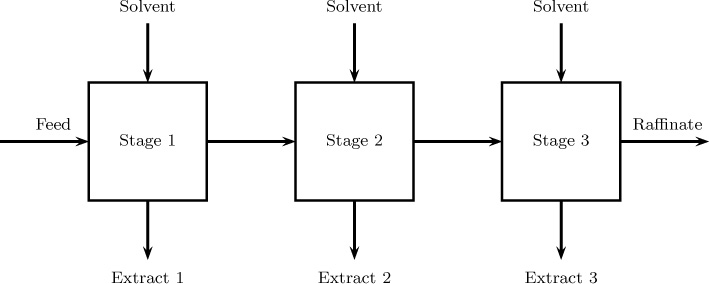
A similar modeling tool applies to multistage separation equipment. Consider liquid–liquid extraction in a mixer-settler as an example. The extent of separation that can be obtained in a single-stage extractor is usually small and multiple units are needed. Usually the system operates in a countercurrent mode, which is known as a multistage cascade. An illustrative sketch is shown in Figure 13.8. Each stage is modeled assuming a backmix–backmix model similar to that studied in Section 13.9.1. Equations are set up for each stage. For a countercurrent operation all the stages have to be solved simultaneously since feed enters at one end and the solvent enters at the other end. For cocurrent cases the model can be solved in a sequential manner.

Diagrammatic representation of multistage cascade.

Three horizontal bars are placed one below the other. Each horizontal bar is divided by two parallel dotted lines, the left segment for Gas and the right for Liquid. Each horizontal bar has an arrow that flows from the left to the right through the dotted parallel lines. The Gas flow direction is from bottom to top indicated by arrows pointing upward, with Gas in at the bottom and the Gas out at the top. Apart from the gas flow, two dotted downward arrows denoting the backflow connect the three bars, the second dotted arrow labeled f subscriptG. The rate of flow of Gas in and Gas out is Q subscriptG, while the concentration of Gas in is C subscript(AG, i) and of the Gas out is C subscript(AG, e). The rate of flow of Gas after passing through the first system from the bottom is Q subscriptG times (1 plus f subscriptG). The Liquid flow direction is from top to bottom indicated by arrows pointing downward, with Liquid in at the top and the Liquid out at the bottom. Apart from the Liquid flow, two dotted upward arrows denoting the backflow connect the three bars, the second dotted arrow labeled f subscriptL. The rate of flow of Liquid in and Liquid out is Q subscriptL, while the concentration of Gas in is C subscript(AL, i) and of the Gas out is C subscript(AL, e). The rate of flow of Liquid after passing through the first system from the top is Q subscriptL times (1 plus f subscriptL).

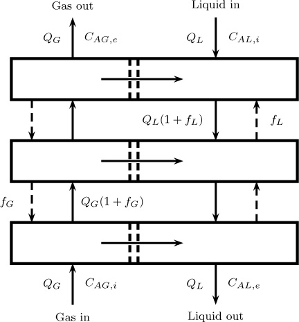
Figure 13.8 Stagewise backmixing model for a two-phase system showing three stages: interstage backflow terms f_L and f_G are often added to provide flexibility to characterize the mixing pattern.

The stages need not be discrete units and this could be done even for a single column. For example, column extractors with various internal design arrangements to provide mechanical agitation are common in industrial practice. Common contactors Scheibel columns of different internal configurations, Oldshue-Rushton columns, rotating disk contactors, and Kuhni columns; these are discussed by Seader et al. (2011). These columns can then be modeded as a number of stages or cascades arranged in a countercurrent manner. In some cases some backflow between stages is included, as shown in Figure 13.8. Equations can then be set up for each stage and the resulting set of algebraic equations can be solved simultaneously to get the exit concentrations and also the various inter-stage concentrations.

13.10.1 Equilibrium Model

For preliminary design an equilibrium model where the streams existing any particular stage are assumed to be in equilibrium is used. For linear equilibrium analytical solutions can be obtained; these are summarized in this section.

Single Stage

The single stage was analyzed in Section 3.8.2. The fractional non-extraction is given by Equation 3.33, which can be expressed as

\frac{X_{e}}{X_{f}} = \frac{1}{1 + E}

$\frac{X_{e}}{X_{f}} = \frac{1}{1 + E}$

where E is called the extraction factor, defined as

E = \frac{S K_{A}}{F_{C}}

$E = \frac{S K_{A}}{F_{C}}$

where S is the solvent rate, F_C is the carrier molar flow rate, and K_A is the equilibrium constant, expressed as mole ratios. This expression assumes that K_A is constant and not a function of composition.

Crosscurrent Cascade

An arrangement used for separations that are not so difficult is the cross-current cascade. The schematic is shown in Figure 13.9. Here fresh solvent is added to each stage and the extracts are collected at the exit of each stage. The fraction of A not extracted is given by the following equation for this case:

\begin{matrix} \frac{X_{Ae}}{X_{Af}} = \frac{1}{(1 + E / N)^{N}} & (13.29) \end{matrix}

$\begin{matrix} \frac{X_{Ae}}{X_{Af}} = \frac{1}{(1 + E / N)^{N}} & (13.29) \end{matrix}$

Diagrammatic representation shows the basic setup of crosscurrent extraction.

Figure 13.9 Schematic of crosscurrent extraction.

In general the countercurrent arrangement provides more extraction than the crosscurent arrangement.

Countercurrent Cascade

The result can be extended to a countercurrent cascade; the following formula (shown without detailed derivation) is useful for practical applications:

\begin{matrix} \frac{X_{Ae}}{X_{Af}} = \frac{E - 1}{E^{N + 1} - 1} & (13.30) \end{matrix}

$\begin{matrix} \frac{X_{Ae}}{X_{Af}} = \frac{E - 1}{E^{N + 1} - 1} & (13.30) \end{matrix}$

This is known as the Kremser equation.

Absorption and Stripping Factors

Similar equations are used for absorption columns. For an N equilibrium stage absorber, with pure absorbent and the streams in counterflow, the recovery fraction is given by the Kremser equation:

ϕ_{A} = \frac{A - 1}{A^{N + 1} - 1}

$ϕ_{A} = \frac{A - 1}{A^{N + 1} - 1}$

where $A$ $A$ is known as the absorber factor and defined as

A = \frac{L}{{Vm}_{A}}

$A = \frac{L}{{Vm}_{A}}$

Here L is the molar liquid flow rate, V is the gas molar flow rate and m_A is the equilibrium constant defined as y = mx.

A similar equation holds for a stripping column. The fraction of species that is not stripped is given as

ϕ_{S} = \frac{S - 1}{S^{S + 1} - 1}

$ϕ_{S} = \frac{S - 1}{S^{S + 1} - 1}$

where S is called the stripped factor, defined as

S = \frac{{Vm}_{A}}{L}

$S = \frac{{Vm}_{A}}{L}$

The stripping factor is the reciprocal of the absorption factor. All three factors, extraction, absorption, and stripping, have similar significance and depend on the linear equilibrium constant times the ratio of the flow rates of the two phases.

Summary

Macroscopic models are derived by using species balances over a large control volume, often the whole reactor or separator. These models lead to algebraic equations rather than differential equations for the steady state case and are therefore easier to solve. They find wide applications in practical design.
An assumption about the mixing pattern in the reactor/separator is needed to assign the kinetic rate and mass transfer driving force terms. A common simplification is that the system is backmixed, which is a reasonable assumption for well-mixed tanks with high levels of agitation. The model is then closed by assuming that the reactor concentration is the same as the exit concentration.
Tracer experiments provide a useful tool to assess the extent of backmixing in the system. For a completely backmixed system for a pulse input of tracer the concentration of the tracer is maximum at time zero and decays as an exponential function. Any deviation of the observed response from this ideal pattern is an indication of less mixing in the system. Such reactors are often modeled as N tanks connected in series. The model parameter to characterize the reactor is N, the number of tanks needed to match the tracer response.
Tracer data can be interpreted in various ways to find the model parameters. Moment analysis is commonly used, where the dimensionless second central moment of the tracer response is matched to the theoretical value. Theoretical values in turn can be generated using the response in the Laplace domain without the need to find the solution in the time domain.
The variance of the response curve is an indicator of the extent of mixing and maldistribution in the reactor. The dimensionless variance is equal to one for a backmixed system. It is equal to zero for plug flow. An intermediate degree of mixing takes a value in between these provided there is no gross maldistribution, recycling, or bypassing. The reactor is then referred to as non-ideal but well behaved.
For reactions with positive order kinetics, plug flow provides the highest conversion and backmixed provides the lowest value. The reactor performance can be bracketed between the high and low values for systems that are well behaved (variance less than one).
Systems with severe maldistribution or bypassing show a variance larger than one. These are called ill-behaved systems. Reactor performance can be even lower that the backmixed case in such situations. An example is a fluidized bed reactor where part of the gas moves as “bubbles” and does not come in contact with catalyst.
For non-first-order reactions, more details on the level of mixing is needed in order to predict reactor performance. The reactor may be well mixed but only on a macro scale. Fluid elements arriving at different times remain segregated in such a situation. The exit age distribution can be used to predict the conversion in a macrofluid model and Equation 13.14 can be used. This provides one bound on the conversion. If the reactor is modeled as a microfluid, we obtain a second bound. Population balance–based models are needed for more detailed modeling of these systems since the level of segregation has to be modeled as well.
Complex systems such as the human body or the environment are often modeled as a network of interconnected compartments and macroscopic balances (usually) are applied to each compartment. Such models find application, for example, in pharmacokinetic modeling to study drug uptake and metabolism. These models are known as compartmental models in general.
An important application of compartmental models is to predict the distribution and fate of chemicals released in the environment. The environment can be considered to be composed of four broad compartments, that is, air, water, soil, and biota (which includes plant and animals). Models of various levels can be used and the primary difference is the level of spatial and component details in each of the compartments. The simplest is the equilibrium model, which is often referred to as a fugacity Level I model.
Separation equipment is often operated in multistage mode; this is known as a cascade arrangement. Commonly countercurrent or crosscurrent cascades are used. Each stage is modeled as a mixed compartment.
The cascades are modeled assuming an equilibrium model at the first level. The mass transfer coefficient and level of mixing is not needed in this model. The extent of separation can then be predicted analytically using the separation factor as a parameter. The number of stages needed to achieve a specified level of separation can be calculated using the expression presented in the text for both the countercurrent and cross-current arrangements.
Equilibrium models can be corrected by using a stage efficiency factor. This depends on the mass transfer coefficient and the mixing pattern in the separator. Analysis for a case where both phases are backmixed is shown in the text.

Review Questions

13.1 If the tracer response is an exponentially decaying function of time, what is the mixing pattern in the reactor?

13.2 If the tracer response is close to a Dirac delta function, what is the mixing pattern in the reactor?

13.3 Can the tracer response to a pulse input show multiple peaks? If so, when?

13.4 Define the E-curve and indicate its physical meaning.

13.5 Define the F-curve and indicate its physical meaning.

13.6 Define the I-curve and indicate its physical meaning.

13.7 What is the expression for the I-curve for a completely mixed reactor?

13.8 A reactor is modeled as four tanks in series. What is the time at which the maximum concentration in the exit for an input of a pulse tracer is observed?

13.9 What is meant by the stiffness factor for a set of first-order differential equations?

13.10 Why is fugacity preferred as the variable in environmental models?

13.11 Which mode gives higher separation: countercurrent or crosscurrent?

13.12 What is the Kremser equation?

13.13 Define absorption, extraction, and stripping factors.

Problems

13.1 Limit for large N for the tanks in series model. What is the limit of expression 13.12 for the concentration in the tanks in series model for N tending to ∞? Show that the plug flow model is approached.

13.2 Reactor performance for the tanks in series model. Calculate and plot the conversion if a reactor is modeled as tanks in series for Da = 3 if the reaction is first order and second order. Take N from 1 to 10. Plot on the same graph the conversion for a plug flow and a backmixed model.

13.3 Response of a tank with a deadzone. A tank is assumed to have a dead zone that exchanges mass with the main zone as shown in Figure 3.10 in Chapter 3. Derive an expression for the response curve in the time domain as well as in the Laplace domain. From the solution derive an expression for the first and second moment and the variance of the response curve.

13.4 Internal age distribution. Show that for a completely backmixed system the I-curve is the same as the E-curve. Thus the probability of an age t in the exit stream is the same as the probability of an age t within the reactor.

13.5 Bolus injection with a first-order reaction. The bolus injection is a very useful and important tool in pharmacokinetic analysis. Repeat the analysis for a bolus injection of tracer that undergoes a first order reaction. Sketch typical exit concentration versus time plots for various values of rate constant (expressed as Da). How is the time constant of the response affected by the rate constant of the reaction?

13.6 Macro- and micro-models for a first-order reaction in a CSTR. For a first-order reaction we have

c_A(t) = exp(–k₁t)

while

E (t) = \frac{1}{\bar{t}} exp (- t / \bar{t})

$E (t) = \frac{1}{\bar{t}} exp (- t / \bar{t})$

where $\bar{t}$ $\bar{t}$ is the mean residence time. Substitute and integrate the macrofluid model given by Equation 13.14. Show that the result is

〈 c_{A, e} 〉 = \frac{1}{1 + k_{1} \bar{t}}

$〈 c_{A, e} 〉 = \frac{1}{1 + k_{1} \bar{t}}$

This is the same as that for a micromixed system. Hence show that for a first-order reaction the level of segregation is not important.

13.7 Macro- and micro-models for a half-order reaction in a CSTR. Compare the macro- and micro-models for a half-order reaction in a CSTR. Use a Damkohler number based on an inlet concentration equal to two.

13.8 Macrofluid model for second-order reaction. For a macro-model the integral given by Equation 13.14 can be integrated analytically, leading to Equation 13.15 in the text. Verify the result.

13.9 Two-compartment versus one-compartment model for drug distribution. The following data was found as a response to a drug that was injected as a pulse. The concentration distribution in the blood was obtained as a function of time. Concentration in the tissue compartment was not measured.

Time	Concentration
0	1.0000
0.3000	0.4867
0.6000	0.2748
0.9000	0.1700
1.2000	0.1101
1.8000	0.0487
2.4000	0.0219

Fit a one-compartment model and determine the time constant. Fit a two-compartment model and find the time constants and the exchange parameter. Comment on the accuracy of the results in view of the fact that the data are limited and no explicit measurement of the tissue concentration was made.

13.10 Pollutant distribution with Level I model. Mackay (2001) studied the distribution of hexachlorobiphenyl (6-CB) in the environment. The molecular weight of this compound is 350 g/gmol, vapor pressure is 0.0033 Pa, and solubility in water is 0.035 g/cm³. The octanol water partition coefficient is 10^6.8. Assume an amount of 5 × 10⁵ mol is dispersed (on an annual basis) in a particular region. Find the distribution in the various compartments. The following values were used for the volumes of each compartment in Mackay’s work: air = 4 × 10¹⁴ m³; water = 2 × 10⁹ m³; soil = 1.2 × 10¹⁰; biota = 8 × 10⁸ m³. The organic carbon in solids is taken as 0.02.

13.11 Extraction efficiency equations. Starting from the basic mass balances coupled with the assumption that the exit streams are in equilibrium, derive Equations 13.30 and 13.29 relating the extent of extraction to the extraction factor. Make a comparison plot between the crosscurrent and countercurrent for extraction factors of 2 and 5.

13.12 Extraction efficiecy of a countercurrent cascade. Water and p-dioxane formed by catalytic dehydration of ethylene glycol are to be separated by liquid–liquid extraction. Since the boiling points of these compounds are very close (100 and 101.1 °C (Seader et al.), distillation is not feasible. Liquid extraction with benzene as a solvent is used. Consider a feed of 4530 kg/hour with a 25% solution of p-dioxane. Benzene and water are mutually insoluble and the distribution coefficient of dioxane (mole ratio in benzene to water) is near 1.2. The flow rate of benzene is 6800 kg/hour. Find the fractional extraction for single-stage and two-stage countercurrent extraction, and two stage crosscurrent extraction. Assume an equilibrium model. If 99% extraction is needed, find the number of counter-current stages that need to be used.

..................Content has been hidden....................

You can't read the all page of ebook, please click here login for view all page.

Table of Contents for Chapter 13. Macroscopic and Compartmental Models

Create new playlist

Sign In

Sign Up

Chapter 13. Macroscopic and Compartmental Models

13.1 Stirred Reactor: The Backmixing Assumption

13.2 Transient Balance: Tracer Studies

13.2.1 Step Input

13.2.2 Pulse or Bolus Input

13.2.3 Age Distribution Functions

E-Curve

F-Curve

I-Curve

13.2.4 Tracer Response for Tanks in Series Model

13.3 Moment Analysis of Tracer Data

13.3.1 Moments from Laplace Transform of Response

13.4 Tanks in Series Models: Reactor Performance

13.5 Macrofluid Models

13.5.1 Second-Order Reaction

13.5.2 Zero-Order Reaction

13.6 Variance-Based Models for Partial Micromixing

13.7 Compartmental Models

13.7.1 Matrix Representation

13.8 Compartmental Models for Environmental Transport

13.8.1 Fugacity of Pollutants in Each Compartment

13.8.2 Level I or Equilibrium Model

13.8.3 Level II Model: Advection Effects

13.8.4 Level III Model: Intermedia Transport Effects

13.8.5 Level IV Model: Transient Effects

13.9 Fluid–Fluid Systems

13.9.1 Backmixed–Backmixed Model

13.9.2 Equilibrium Model

13.9.3 Mixing Cell Model

13.10 Models for Multistage Cascades

13.10.1 Equilibrium Model

Single Stage

Crosscurrent Cascade

Countercurrent Cascade

Absorption and Stripping Factors

Summary

Review Questions

Problems

Table of Contents for
Chapter 13. Macroscopic and Compartmental Models