Chapter 17. Laminar Flow Reactor

Search in book...
Toggle Font Controls
Create new playlist

Name your new playlist

Playlist description (optional)
Sign In

Email address

Password

Forgot Password?

or

Continue with Facebook

Continue with Google
Sign Up

Full Name

Email address

Confirm Email Address

Password

or

Continue with Facebook

Continue with Google

Chapter 17. Laminar Flow Reactor

Learning Objectives

After completing this chapter, you will be able to:

Apply differential equations of mass transfer to laminar flow with homogeneous and heterogeneous reactions.
Render the equation to a dimensionless form and identify the key dimensionless groups.
Solve the equation by a number of mathematical and computational tools.
Identify two limiting cases of the model, that is, the segregated flow and the plug flow model.
Compare the mesoscopic approach based on the dispersion model with the exact 2-D model, segregated model, and plug flow model.
Examine briefly the temperature effect in a laminar flow reactor and modeling of a turbulent flow reactor.

Reactors under laminar flow conditions are often encountered in industrial practice, especially for viscous liquids. The modeling of such systems involves the convection-diffusion equation for mass transfer together with homogeneous and, in some cases, wall catalyzed heterogeneous reactions. Study of such systems is thus important not only in reaction engineering but also in mass transfer analysis. The chapter can be viewed as a case study example of this analysis. We first formulate a full 2-D model, identify the key dimensionless groups, and show some numerical solutions. These solutions will then be used as benchmarks to examine some approximate limiting cases.

Two simplified limiting models are often used. These are a pure convection model and a plug flow model. In the convection model it is assumed that there is no radial diffusion (which is relatively small and therefore neglected) and each fluid element slides past each other with no interaction by molecular diffusion. In the second model, the radial diffusion is rapid and the concentration variation across the radial direction is not assumed to exist; therefore the system is close to plug flow conditions. From this qualitative discussion, you can guess that the convection model applies when the diffusion coefficient is small.

Another approach is to use the dispersion model in conjunction with a mesoscopic model. We compare these various models and this enables you to get a good conceptual understanding of the interplay of the various transport mechanisms involved in the system.

The focus is mainly on isothermal systems with Newtonian flow. This is the simplest example of a laminar flow reactor, enables you to understand the modeling approach, and permits you to extend to other cases. A few examples of complex cases are mentioned in this chapter but not studied in detail. These are non-Newtonian fluids, turbulent flow, and non-isothermal systems. Some additional references are provided so that the interested reader can pursue further study of these topics.

17.1 Model Equations and Key Dimensionless Groups

Consider a fully developed flow of a Newtonian fluid in a circular pipe. The fluid is a mixture containing a compound A at a concentration of C_A,i at the inlet. This compound undergoes a chemical reaction in the system with a rate constant of k. The reaction is assumed to be first order. Also the walls are coated with a catalyst and the compound A reacts at the wall with a surface reaction constant of k_S.

The goal is to examine and solve the model differential equation and to obtain the concentration distribution of A as a function of both z, the axial distance from the entrance, and r, the radial coordinate. We assume the concentration is symmetric in the θ direction in cylindrical coordinates.

17.1.1 Dimensionless Model Equations

The differential equation for concentration distribution of species A as a function of r and z given by the convection-diffusion-reaction (CDR) model. The model is given by the following equation:

\begin{matrix} 2 〈 υ 〉 (1 - {(r / R)}^{2}) \frac{\partial C_{A}}{\partial z} = D [\frac{\partial^{2} C_{A}}{\partial z^{2}} + \frac{1}{r} \frac{\partial}{\partial r} (r \frac{\partial C_{A}}{\partial r})] - k C_{A} & (17.1) \end{matrix}

$\begin{matrix} 2 〈 υ 〉 (1 - {(r / R)}^{2}) \frac{\partial C_{A}}{\partial z} = D [\frac{\partial^{2} C_{A}}{\partial z^{2}} + \frac{1}{r} \frac{\partial}{\partial r} (r \frac{\partial C_{A}}{\partial r})] - k C_{A} & (17.1) \end{matrix}$

In this equation a parabolic velocity profile has been used, which is valid for a Newtonian fluid. D is the diffusion coefficient of A. The reaction is assumed to be first order. If the reaction is not first order the rate term kC_A is replaced by some “rate” function of C_A and the differential equation becomes nonlinear. We consider only the linear case and the nonlinear case is left as a computational exercise.

The following dimensionless variables are introduced:

Dimensionless radial position ξ = r/R.
Dimensionless concentration c_A = C_A/C_A,i.
Dimensionless axial length η = z/L; here L is some specified length of the reactor and the variable η goes from 0 to 1 (entrance and exit of the reactor, respectively).

The axial diffusion term in Equation 17.1 (the first term in the square bracket on the right-hand side) can usually be neglected. This is similar to the case of mass transfer with no reaction examined in Section 10.1 and is justified if the Peclet parameter is greater than, say, 10. In dimensionless form the following equation will then be obtained:

\begin{matrix} 2 (1 - ξ^{2}) \frac{{\partial c}_{A}}{\partial η} = \frac{L}{R} \frac{1}{P e_{R}} [\frac{1}{ξ} \frac{\partial}{\partial ξ} (ξ \frac{{\partial c}_{A}}{\partial ξ})] - {D a c}_{A} & (17.2) \end{matrix}

$\begin{matrix} 2 (1 - ξ^{2}) \frac{{\partial c}_{A}}{\partial η} = \frac{L}{R} \frac{1}{P e_{R}} [\frac{1}{ξ} \frac{\partial}{\partial ξ} (ξ \frac{{\partial c}_{A}}{\partial ξ})] - {D a c}_{A} & (17.2) \end{matrix}$

The dimensionless numbers appearing here are the Damkohler number, the Peclet number, and the length to radius ratio. The Damkohler number Da is defined as

Da = kL/〈υ〉

and the Peclet number Pe_R (using radius as a length scale) is defined as

Pe_R = 〈υ〉 R/D

The length to tube radius ratio, which is the third parameter, can be combined with Pe_R to get a composite dimensionless group B defined as (L/R)/Pe_R.

Note: We use the tube radius as the representative length to define the Peclet number while the diameter was used in Chapter 10. The subscript R on the Peclet number is used to distinguish this defnition.

Time Scales

Four time scales can be defined as indicated in a seminal work by Chakraborty and Balakotaiah (2002). These time scales are:

Mean residence $= \frac{L}{< υ >}$ $= \frac{L}{< υ >}$
Reaction $= \frac{1}{k_{1}}$ $= \frac{1}{k_{1}}$ for a first-order reaction or $\frac{1}{k_{n} C_{A i}^{n - 1}}$ $\frac{1}{k_{n} C_{A i}^{n - 1}}$ for a nth-order reaction.
Radial diffusion time $= \frac{R^{2}}{D_{A}}$ $= \frac{R^{2}}{D_{A}}$
Axial diffusion time $= \frac{L^{2}}{D_{A}}$ $= \frac{L^{2}}{D_{A}}$

One should estimate the values of these time constants and the reactor performance will not depend on the phenomena having large time constants. (The effect of axial diffusion is usually neglected since the axial diffusion time is relativity larger compared to other time scales in this system.)

Note that due to low values of the diffusion coefficient in the liquid phase (compared to the gas phase), the radial diffusion time is quite large in liquid. Hence the effect of radial diffusion can often be neglected for liquids, but this may not be so for gases in small diameter tubes as shown in an early and seminal work by Cleland and Wilhelm (1956).

Relation of the Dimensionless Groups to the Time Constants

It is also useful to write the dimensionless groups as the ratio of time constants.

The dimensionless group Pe_R has the following significance:

{P e}_{R} = \frac{Mass transport by convection}{Mass transport by diffusion}

${P e}_{R} = \frac{Mass transport by convection}{Mass transport by diffusion}$

It can be shown to be propotional to the ratio of the radial diffusion time to the convection time.

Likewise Da can be shown to be the ratio of the residence time to the reaction time:

D a = \frac{L / 〈 υ 〉}{1 / k} = \frac{Residence time}{Reaction time}

$D a = \frac{L / 〈 υ 〉}{1 / k} = \frac{Residence time}{Reaction time}$

Finally the group appearing at the front of the right-hand side of Equation 17.2, denoted as B, can be shown to be

B = \frac{L}{R} \frac{1}{{P e}_{R}} = \frac{L / 〈 υ 〉}{R^{2} / D} = \frac{mean residence time}{radial diffusion time}

$B = \frac{L}{R} \frac{1}{{P e}_{R}} = \frac{L / 〈 υ 〉}{R^{2} / D} = \frac{mean residence time}{radial diffusion time}$

This group plays an important role in determining the importance of the radial diffusion. It is the ratio of time spent by fluid in the reactor (on average) to the time it takes for the diffusion to equalize the radial variation in concentration. If this parameter is large, radial diffusion time is small and the concentration is likely to be equalized in the radial direction. Plug flow behavior can be expected. Results shown later will verify this effect.

On the contrary if the B parameter is small, the radial diffusion time is large and the radial diffusion is not likely to start to click in during the mean passage time of the fluid. Fluid elements at each radial position will behave as though they are flowing independently of each other and the segregated flow model is expected to be applicable.

17.1.2 Boundary Conditions

At the inlet η = 0 we set c_A = 1. At the center ξ = 0 we have symmetry and therefore ∂c_A/∂ξ = 0.

The boundary condition at the wall in the presence of a heterogeneous wall reaction is of the Robin type and can be expressed as

\begin{matrix} (\frac{{\partial c}_{A}}{\partial ξ})_{ξ = 1} = - B i_{w} c_{A} at ξ = 1 & (17.3) \end{matrix}

$\begin{matrix} (\frac{{\partial c}_{A}}{\partial ξ})_{ξ = 1} = - B i_{w} c_{A} at ξ = 1 & (17.3) \end{matrix}$

Thus an additional dimensional parameter, wall reaction Biot number, Bi_w = k_wR/D_A_–_m, arises for this problem. This group can be shown to signify the relative ratio of the radial diffusion time to the surface reaction time.

No flux condition can be used for the case of no wall reaction, leading to a Neumann condition. Further if the surface reaction is extremely rapid, the concentration at the wall can be set to zero, leading to a Dirichlet problem. Hence it is interesting to note that all three common conditions arise for this problem depending on the wall condition.

The result of dimensionless formulation thus leads to the following parametric representation of the problem:

c_A = c_A(η, ξ, ; B, Da, Bi_w)

A numerical solution can be readily obtained using the PDEPE software.

The results are usually represented in terms of a cup-mixing average concentration, which is defined as

\begin{matrix} c_{Ab} (η) = 4 \int_{0}^{1} ξ (1 - ξ^{2}) c_{A} (ξ) d ξ & (17.4) \end{matrix}

$\begin{matrix} c_{Ab} (η) = 4 \int_{0}^{1} ξ (1 - ξ^{2}) c_{A} (ξ) d ξ & (17.4) \end{matrix}$

Usually the value of the cup-mixing concentration at the exit (η = 1) is the quantity of design interest. Note conversion equals 1 – c_Ab at η = 1.

Limiting cases of the model are now examined.

17.2 Two Limiting Cases

This section examines two limiting cases that depend on the value of parameter B and develops a simplified solution for these limiting cases.

Parameter B, which appears in the front of the radial diffusion term, can be written as

B = \frac{L}{< υ >} \frac{D}{R^{2}} = \bar{t} (D / R^{2})

$B = \frac{L}{< υ >} \frac{D}{R^{2}} = \bar{t} (D / R^{2})$

Observe that this is the ratio of mean residence time to the diffusion time in the radial direction. Equation 17.2 can be written as

\begin{matrix} 2 (1 - ξ^{2}) \frac{{\partial c}_{A}}{\partial η} = B [\frac{1}{ξ} \frac{\partial}{\partial ξ} (ξ \frac{{\partial c}_{A}}{\partial ξ})] - {D a c}_{A} & (17.5) \end{matrix}

$\begin{matrix} 2 (1 - ξ^{2}) \frac{{\partial c}_{A}}{\partial η} = B [\frac{1}{ξ} \frac{\partial}{\partial ξ} (ξ \frac{{\partial c}_{A}}{\partial ξ})] - {D a c}_{A} & (17.5) \end{matrix}$

Some limiting cases will now be analyzed depending on the value of the B parameter. It is useful to have a full 2-D solution at hand to compare the limiting cases, which can be simulated using the MATLAB tool PDEPE. An illustrative result is shown in Figure 17.1 as a plot of c_Ab(exit) versus B for a fixed Da = 3. These results are useful in understanding the role of radial diffusion. We discuss the limiting cases of small B and large B now.

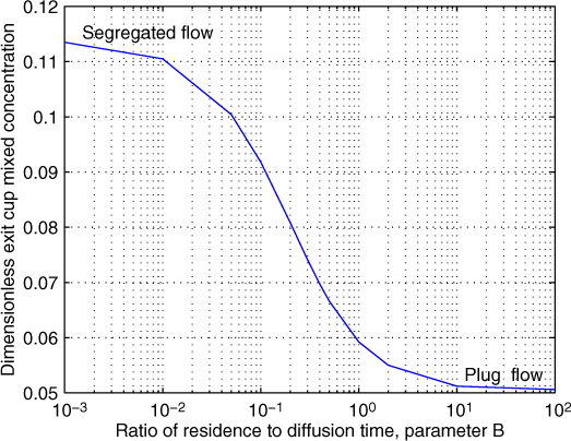
A line graph of dimensionless exit cup mixed concentration versus parameter B.

Figure 17.1 Effect of radial diffusion on performance of a laminar flow reactor; results are for Da = 3.0.

17.2.1 Small B: Pure Convection Model

If the B parameter is small then the radial diffusion term can also be dropped in Equation 17.5, leading to a model called a pure convection model, also known as the segregated flow model. A value of B < 5 × 10^–3 was suggested by Merrill and Hamrin (1970) for liquid phase systems as an approximate criteria.

The segregated model has a simple representation by dropping the B term in Equation 17.5:

\begin{matrix} 2 (1 - ξ^{2}) \frac{{\partial c}_{A}}{\partial η} = - {D a c}_{A} & (17.6) \end{matrix}

$\begin{matrix} 2 (1 - ξ^{2}) \frac{{\partial c}_{A}}{\partial η} = - {D a c}_{A} & (17.6) \end{matrix}$

The model can be readily solved and integrated over the cross-section to model reactor performance. The concentration at any radial position is obtained as

c_{A} (ξ) = exp (- \frac{Daη}{2 (1 - ξ^{2})})

$c_{A} (ξ) = exp (- \frac{Daη}{2 (1 - ξ^{2})})$

The reactor exit is at η = 1 and the exit concentration profile can be computed. The cup-mixing exit concentration can be then evaluated. An illustrative exit profile is shown in Figure 17.2.

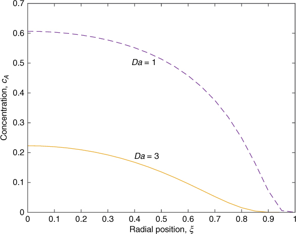
A line graph of concentration versus radial position, showing two curves representing first order reaction.

Figure 17.2 Exit radial concentration profile in a laminar flow reactor on the basis of the segregated flow model; results for Da = 1.0 and Da = 3.0 for first-order reaction.

Note that the center has higher concentration since the fluid elements at the center have spent only half the mean residence time. For example, for Da = 1, the center concentration is exp(–Da/2) = 0.6035. The wall concentration is zero. Note that the diffusion will act as an equalizer and spread these concentration profiles a bit, but in the segregated flow model the radial diffusion is assumed to be absent.

Knowing the radial distribution of the concentration it remains to find the cup-mixing concentration by radial integration as per Equation 17.4. The final result can be expressed as an exponential integral:

\begin{matrix} c_{A b} (exit) = \frac{{D a}^{2}}{4} expint (D a / 2) + (1 - D a / 2) exp (- D a / 2) & (17.7) \end{matrix}

$\begin{matrix} c_{A b} (exit) = \frac{{D a}^{2}}{4} expint (D a / 2) + (1 - D a / 2) exp (- D a / 2) & (17.7) \end{matrix}$

where expint denotes the exponential integral.

17.2.2 Large B: Plug Flow Model

A second limiting case is the plug flow model for large B, which results after some cross-sectional averaging of Equation 17.5. The exit concentration is given as

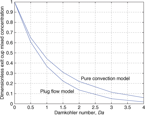
\begin{matrix} c_{A b} (exit) = exp (- D a) & (17.8) \end{matrix}

$\begin{matrix} c_{A b} (exit) = exp (- D a) & (17.8) \end{matrix}$

Figure 17.3 shows a comparison of these limiting case for various values of Da. The difference starts to appear at larger values of Da, that is, for large reactor conversions. The reactor performance can be bracketed between the limits of the segregated model and plug flow model. For example, if Da = 3 the segregated model gives a conversion of 89% while the plug flow model gives a conversion of 95%.

A line graph showing the comparison of pure convection model and plug flow model.

Figure 17.3 Comparison of pure convection and the plug flow model for laminar flow reactor.

The dispersion model based on a mesoscopic average is also used and we now present and show some results for this model.

17.3 Mesoscopic Dispersion Model

Sections 14.2 and 14.3 should be reviewed at this stage. A few concepts are, however, repeated here for ease of understanding.

If the B parameter is in the intermediate range, neither the segregated model nor the plug flow model will be reasonable. There is some smearing of concentration in the radial direction. The full 2-D model should be used for such cases. However, the model can be reduced to a 1-D or mesoscopic model by radial averaging, which is taken up in the following section. The radial averaging needs additional closure terms, which are determined using the Taylor dispersion model. The resulting 1-D model for the reactor is known as the axial dispersion model. These concepts were already introduced in Section 4.2.2 and Section 14.2 and these sections should be reviewed at this stage.

For laminar flow the dispersion coefficient can be obtained from the theory derived by Taylor. The equation for the dispersion coefficient was presented in Section 14.4 and with some rearrangement of the equation, we have the following relation for the dispersion number:

\begin{matrix} D_{E}^{*} = \frac{1}{48 B} & (17.9) \end{matrix}

$\begin{matrix} D_{E}^{*} = \frac{1}{48 B} & (17.9) \end{matrix}$

The reciprocal of $D_{E}^{*}$ $D_{E}^{*}$ is defined as the dispersion Peclet number:

P e * = \frac{1}{D_{E}^{*}} = 48 B

$P e * = \frac{1}{D_{E}^{*}} = 48 B$

In terms of the dispersion Peclet number the dispersion model is written as

\begin{matrix} \frac{1}{P e *} \frac{d^{2} < c >}{d η^{2}} - \frac{d < c >}{dη} - Da < c > = 0 & (17.10) \end{matrix}

$\begin{matrix} \frac{1}{P e *} \frac{d^{2} < c >}{d η^{2}} - \frac{d < c >}{dη} - Da < c > = 0 & (17.10) \end{matrix}$

Danckwerts boundary conditions are commonly used in the context of the dispersion model. In the previous equation, < c > is the cross-sectional average concentration of species A.

The result for the average concentration for a first-order reaction using the above-stated boundary condition was given in Section 14.2.1. Please review this section at this stage. The results are summarized in the following for easy reference:

\begin{matrix} < c > (η = 1) = \frac{4 α exp (P e * / 2)}{{(1 + a)}^{2} exp (α P e * / 2) - {(1 - a)}^{2} exp (- α P e * / 2)} & (17.11) \end{matrix}

$\begin{matrix} < c > (η = 1) = \frac{4 α exp (P e * / 2)}{{(1 + a)}^{2} exp (α P e * / 2) - {(1 - a)}^{2} exp (- α P e * / 2)} & (17.11) \end{matrix}$

where

α = \sqrt{(1 + 4 Da / P e *)}

$α = \sqrt{(1 + 4 Da / P e *)}$

The effect of the B parameter is examined now based on the dispersion model. For each B parameter the value of Pe* is equal to 48 B. The exit concentration is then calculated using Equation 17.11. The results are compared in Table 17.1. Results for the exit concentration are compared for various values of the relative diffusion parameter, B, for a fixed value of Da equal to 3.

Table 17.1 Comparison of the Dispersion Model with the Detailed 2-D Model for Da = 3

B values	0.01	0.1	1.0	10.0
Pe* values	0.48	4.8	48.0	480.0
〈c_A〉 (1) 2-D model	0.1102	0.0915	0.0587	0.0507
〈c_A〉 (1) Dispersion model	0.2134	0.1123	0.0587	0.0507

The following conclusions are useful to note. The dispersion model should not be used if the B parameter is less than 0.1. For such cases the dispersion model results are closer to the backmixed reactor model rather than to the more realistic segregated flow model. For large values of B > 1 there is hardly any difference between the dispersion model and the full-D model. Plug flow is nearly achieved as well. Thus the dispersion model is useful for the intermediate range of the relative diffusion parameter, that is, for 0.1 < B < 1.0.

17.4 Other Examples of Flow Reactors

The previous sections provided a complete treatment of a laminar reactor in a pipe flow for a Newtonian fluid. A full 2-D model, dispersion model, segregated flow model, and plug flow model were compared and the range of validity of each model was discussed. In this section, we present some discussion on flow reactors for some other useful cases.

17.4.1 Channel Flow

Channel flow is encountered in some applications, for example, microchannel reactors, monoliths with catalytic walls, and so on. The system is simulated using the appropriate velocity profile and Laplacian in Cartesian coordinates. The governing differential equation is

\begin{matrix} \frac{3}{2} 〈 υ 〉 [1 - {(y / H)}^{2}] \frac{\partial C_{A}}{\partial x} = D \frac{\partial^{2} C_{A}}{\partial y^{2}} - k C_{A} & (17.12) \end{matrix}

$\begin{matrix} \frac{3}{2} 〈 υ 〉 [1 - {(y / H)}^{2}] \frac{\partial C_{A}}{\partial x} = D \frac{\partial^{2} C_{A}}{\partial y^{2}} - k C_{A} & (17.12) \end{matrix}$

A parabolic velocity profile has been used here that is valid for a Newtonian fluid. The wall boundary conditions can be appropriately defined depending on whether there is a wall reaction or not. The PDEPE solver is useful to compute this with only minor changes in the various definitions. If the dispersion model is used (which again is useful in the intermediate range of the B parameter) the dispersion coefficient to be used is given in Section 14.6.

17.4.2 Non-Newtonian Fluids

Many important practical systems (e.g., polymerization reactions) obey the non-Newtonian model for fluid behavior. A power law model is often used for the stress-strain rate relation. In such cases the velocity profile is given as

\begin{matrix} υ_{z} = \frac{3 n + 1}{n + 1} 〈 υ 〉 [1 - (\frac{r}{R})^{(n + 1) / n}] & (17.13) \end{matrix}

$\begin{matrix} υ_{z} = \frac{3 n + 1}{n + 1} 〈 υ 〉 [1 - (\frac{r}{R})^{(n + 1) / n}] & (17.13) \end{matrix}$

Numerical solutions can be obtained by PDEPE using this velocity profile. The effect of the power law index on reactor performance can then be examined. Illustrative results are presented in Table 17.2.

Table 17.2 Effect of Power Law Index on the Performance of a Laminar Flow Reactor

B values	0.01	0.1	1.0	10.0
n = 1	0.1102	0.0915	0.0587	0.0507
n = 0.5	0.0948	0.0791	0.0559	0.0504

In Table 17.2 the results for the exit concentration are compared for various values of the relative diffusion parameter, B. The value of Da was set as 3. For B > 1, the power law index parameter does not appear to be important since the system is moving toward plug flow. For low values of B, the segregated model can be used and Novosad and Ulbrecht (1966) provide useful results for this case. Hence the modeling approach and the observations for Newtonian flow are still valid and only minor modifications are needed to model the non-Newtonian case. Pure convection models for laminar flow are studied by Osborne (1975), which is a useful additional reference.

An alternative is the dispersion model. This will be useful in the intermediate range of the B parameter. The dispersion coefficient is given by the equation of Fan and Huang (1975):

P e * = \frac{2 (3 n + 1) (5 n + 1)}{n^{2}} B

$P e * = \frac{2 (3 n + 1) (5 n + 1)}{n^{2}} B$

Equation 17.11 can then be used with this value for Pe* for a first-order reaction.

17.4.3 Heat Transfer Effects

Temperature effects are handled by using the analogous heat transfer equation:

\begin{matrix} 2 〈 υ 〉 ρ c_{p} (1 - (r / R)^{2}) \frac{\partial T}{\partial z} = k \frac{1}{r} \frac{\partial}{\partial r} (r \frac{\partial T}{\partial r}) + k_{1} (T) C_{A} (- Δ H_{R}) & (17.14) \end{matrix}

$\begin{matrix} 2 〈 υ 〉 ρ c_{p} (1 - (r / R)^{2}) \frac{\partial T}{\partial z} = k \frac{1}{r} \frac{\partial}{\partial r} (r \frac{\partial T}{\partial r}) + k_{1} (T) C_{A} (- Δ H_{R}) & (17.14) \end{matrix}$

Here k₁, the rate constant, is a function of temperature according to the Arrhenius relation. k is the thermal conductivity of the fluid.

Simultaneous solution of the concentration equation and the temperature equation is needed. The commonly used assumptions are no axial conduction of heat and no change in viscosity, The coupled equations can be easily set up in MATLAB with PDEPE. Churchill and Yu (2006) also provide some numerical solutions and indicate that the computer implementation and solution of such coupled models are within the capability of ordinary desktop computers.

A more general case where the variation of viscosity is important as well as multiple reactions, and so on, requires a detailed solution. Fluid velocity has to be computed simultaneously due to visocity variation with temperature. Hence this is an example of a problem where all three transports (momentum, heat, and mass) are involved. COMSOL-based tutorials are available on the web and these may be useful for such complex situations. A detailed and useful study of the industrially important styrene polymerization reaction is presented in Wyman and Carter (1976). This is a system with large heat effects and significant change in viscosity as one goes from the monomer at the entrance to a polymeric fluid at the exit of the reactor, if all goes well. The system can become unstable for larger tube diameters and for large inlet temperatures and the mathematical models provide us the tools to identify the stable regions of operation. Simulation models have proven to be of great value in safe operation of such reactors in addition to fixing the optimum operating conditions for the reactor.

17.4.4 Turbulent Flow Reactor: 2-D Model

2-D models for turbulent flow can be set up in a similar manner. The key points to note are that the velocity and the concentration should be interpreted as time-averaged values. The diffusion coefficient is also augmented by adding the eddy diffusivity, D_t. The model representation in terms of the time-averaged quantities is

\begin{matrix} {\bar{υ}}_{z} (r) \frac{\partial {\bar{C}}_{A}}{\partial z} = \frac{1}{r} \frac{\partial}{\partial r} (r (D + D_{t}) \frac{\partial {\bar{C}}_{A}}{\partial r}) - k {\bar{C}}_{A} & (17.15) \end{matrix}

$\begin{matrix} {\bar{υ}}_{z} (r) \frac{\partial {\bar{C}}_{A}}{\partial z} = \frac{1}{r} \frac{\partial}{\partial r} (r (D + D_{t}) \frac{\partial {\bar{C}}_{A}}{\partial r}) - k {\bar{C}}_{A} & (17.15) \end{matrix}$

The velocity profile can be approximated by the 1/7th power law as a simplification:

υ_{z} (r) = \frac{60}{49} 〈 υ 〉 [1 - (r / R)]^{1 / 7}

$υ_{z} (r) = \frac{60}{49} 〈 υ 〉 [1 - (r / R)]^{1 / 7}$

An alternative is to use the Prandlt universal velocity profile. Note that the velocity in turbulent flow is a steep function of radius in contrast to the smooth parabolic function characteristic of laminar flow of Newtonian fluid.

The eddy diffusion coefficient is also a function of position and hence is retained inside the derivative sign in Equation 17.15. The following relation for turbulent stress and eddy viscosity proposed by Pai (1953) is useful:

\begin{matrix} τ_{rz}^{(t)} = μ_{t} \frac{\partial υ_{z}}{\partial r} = 0.9835 ρ υ_{f}^{2} (1 - \frac{y^{+}}{H^{+}}) [1 - (1 - \frac{y^{+}}{H^{+}})^{30}] & (17.16) \end{matrix}

$\begin{matrix} τ_{rz}^{(t)} = μ_{t} \frac{\partial υ_{z}}{\partial r} = 0.9835 ρ υ_{f}^{2} (1 - \frac{y^{+}}{H^{+}}) [1 - (1 - \frac{y^{+}}{H^{+}})^{30}] & (17.16) \end{matrix}$

where υ_f is the friction velocity. y⁺ is the dimensionless distance measured from the wall. The turbulent diffusivity is then calculated as ν_t/Sc_t with a value of 0.9 assigned for Sc_t, the turbulent Schmidt number.

Further complexity arises for non-first-order reactions. Additional contribution due to the fluctuating concentration results in the rate term. For example, for a second-order reaction an additional rate term k₂ < C′_A > ² is needed. However, these effects can usually be neglected, except for gas phase reactions at high temperature, as pointed out by Glassman (1966).

Detailed computations of tubular reactors under turbulent flow conditions have been done by Yu and Churchill (2006). They provide useful benchmark results for comparison of the numerical tools, which may be useful for solution of the governing equations. They found that the central finite difference is fairly accurate and also indicate that these days, the numerical study of these type of problems is entirely within the capacity of undergraduate students.

Most CFD codes have provision for simultaneous solution of the velocity profile and the concentration profile. COMSOL-based simulation modules are also available.

17.4.5 Axial Dispersion Model for the Turbulent Case

A simplified model is obtained by using the axial dispersion model. The correlation for an axial dispersion coefficient in turbulent flow is discussed in Section 14.6, and it can be used to predict conversion in the reactor (see Ramachandran and Mashelkar (1976), for detailed numerical results on the effect of axial dispersion on the performance of a turbulent flow reactor).

In general the departure from plug flow is small unless the reactor is operated at high conversion levels. The following criteria was suggested by Ramachandran and Mashelkar to estimate the deviation from plug flow:

\begin{matrix} \frac{c_{A}}{c_{A, p}} = 1 + R e^{- 1 / 8} \frac{d_{t}}{〈 υ 〉} \frac{R_{A} (C_{A, p})}{C_{A, p}} \ln [\frac{R_{A} (C_{A, p})}{R_{A} (C_{A, i})}] & (17.17) \end{matrix}

$\begin{matrix} \frac{c_{A}}{c_{A, p}} = 1 + R e^{- 1 / 8} \frac{d_{t}}{〈 υ 〉} \frac{R_{A} (C_{A, p})}{C_{A, p}} \ln [\frac{R_{A} (C_{A, p})}{R_{A} (C_{A, i})}] & (17.17) \end{matrix}$

Here c_A,p is the concentration if plug flow existed. Equation 17.17 is based on the Blasius correlation for the friction factor, the Taylor model for dispersion in turbulent flow, and the perturbation analysis of the dispersion model done by Horn and Parish (1967) to study small deviation effects from plug flow.

For a first-order reaction this reduces to

\frac{c_{A}}{c_{A, p}} = 1 - R e^{- 1 / 8} \frac{d_{t}}{L} D a^{2}

$\frac{c_{A}}{c_{A, p}} = 1 - R e^{- 1 / 8} \frac{d_{t}}{L} D a^{2}$

For example if Da = 3 and Re = 5000, the ratio is 0.969 for an L/d_t ratio of 100. The conversion values would be only 3% lower, showing that the deviation from plug flow is not significant even at this conversion level.

Summary

An important application of the convective transport equations is in the simulation of the laminar flow reactor. A 2-D model shows that the Damkohler number and modified Peclet number (B parameter) are the key dimensionless groups that influence reactor performance.
A laminar flow model can be simplified in some cases where the radial diffusion term is small. This holds when the B parameter is small and leads to a model called the pure convection model. If the velocity variation is neglected, the reactor can be modeled as a plug flow model. This will hold for large B. These two models provide two limiting cases for the complete 2-D laminar reactor model.
The dispersion model can also be used to model the performance of the laminar flow reactor. This model predicts the laminar reactor performance in the intermediate range of values for B. The dispersion model should not be used if the B parameter is small, say less than 0.1. In such cases the segregated flow model should be used.
A detailed 2-D model can be solved numerically and code based on the PDEPE solver given in the text in Section 8.11 can be adapted to simulate the reactor. This is useful for a variety of similar applications, for example, channel flow, non-Newtonian fluids, turbulent flow, and exothermic reactions (where simultaneous solution of the heat equation is needed). Both homogeneous reaction in the bulk fluid and heterogeneous reaction on the wall coated with a catalyst can be simulated by this numerical tool.
Heat effects can be included by adding an additional heat equation for the temperature profile and incorporating the Arrhenius law for the effect of temperature on the rate constant. The coupling can be strong for highly exothermic reactions and can lead to numerical difficulties in the solution. The reactor can show instability and temperature run-away. The identification of safe regions of operation using model-based computations is extremely important in control of such exothermic reactors.
Turbulent flow reactors need additional model closures. The velocity profile needs to be modified and a profile for turbulent diffusivity must be included in the species mass conservation equation. In general turbulent reactors are close to plug flow unless high conversions (>95%) are encountered.

Review Questions

17.1 Define the relative diffusion parameter, B, and express this as a ratio of two time constants.

17.2 What is the role of the B parameter in determining which type of model to use for the laminar flow reactor?

17.3 When will the plug flow model apply to a laminar flow reactor?

17.4 When will the segregated flow model (pure convection model) apply for a laminar flow reactor?

17.5 When would you use the dispersion model for laminar flow?

17.6 Under what conditions would you not use the dispersion model to simulate a laminar flow reactor?

17.7 What additional parameters are needed to model a turbulent flow reactor?

Problems

17.1 Conversion in laminar flow reactor. An aqueous solution containing a reactant A is flowing in laminar flow in a reactor and undegoes a first-order reaction with a rate constant of 0.5 s^–1. The physical properties are the same as water and the diffusion coefficient is estimated as 2 × 10^–9 m²/s. The tube diameter is 50 mm, the length is 3 m, and the average velocity is 0.1 m/s. Find the conversion based on a full 2-D simulation. PDEPE is directly useful here.

17.2 Time constants and model to use. In the previous problem estimate the various time constants and state what type of simpler 1-D model would be most appropriate rather than a full 2-D numerical simulation.

17.3 Second-order reaction. For the same conditions find the conversion if the reaction is second order with a rate constant of 2.5 × 10^–4 m³/mol s.

17.4 Comparision of plug flow and laminar flow. A reactor gives a conversion of 95% if operated as a plug flow. But the fluid is highly viscous and laminar flow is applicable. What would be the conversion in the reactor?

17.5 Pure convection model: zero-order reaction. Extend the analysis of the pure convection model shown in Section 17.1.1 to a zero-order reaction. Verify the following equation for the conversion given by Levenspiel (1999):

c_{A} (exit) = {(1 - \frac{D a}{2})}^{2}

$c_{A} (exit) = {(1 - \frac{D a}{2})}^{2}$

where Da is the Damkohler number for a zero-order reaction. How is it defined? Find the length for complete conversion for a zero-order reaction based on the above model if the length needed is 3 m for a plug flow situation.

17.6 Pure convection model: second-order reaction. Extend the analysis in Section 17.1.1 to a second-order reaction. Verify the following equation for the conversion given by Levenspiel (1999):

c_{A} (exit) = 1 - D a [1 - \frac{D a}{2} ln (1 + \frac{2}{D a})]

$c_{A} (exit) = 1 - D a [1 - \frac{D a}{2} ln (1 + \frac{2}{D a})]$

where Da is the Damkholer number for a second-order reaction. How is it defined?

17.7 Multiple reactions. Set up the model for a series reaction taking place in a pipe under laminar flow conditions:

A → B → C

Solve with PDEPE and compare the limiting cases of the convection model and the plug flow model. Because of the velocity profile, the maximum concentration of the intermediate species, B, will be less than that for a plug flow reactor. Verify this observation.

17.8 Non-Newtonian fluids. Consider a fluid with a power law index of 0.5. The value of the relative diffusion parameter, B, is 0.6. The Damkohler number is 3. Compare the 2-D model with the axial dispersion model.

17.9 Laminar flow in a channel with wall reaction. Often wall-coated channels are used in pollution abatement. In such cases there is no homogeneous reaction and the wall reaction is the dominant term. Set up and solve the 2-D model for the following conditions: channel width = 5 mm; channel length = 2 m; average velocity = 5 cm/s, wall rate constant = 10^–4 m/s; D = 2 × 10^–4 m²/s. An alternative is to use the mesoscopic model. Set up this model as well and compare the predictions.

17.10 Homogeneous and heterogeneous reactions. Solve the laminar flow reactor where both homogeneous and heterogeneous reactions are taking place for the following values of the dimensionless parameters: B = 1.0; Da = 4; Bi_w = 2.0. Find the cup-mixing concentration at the exit of the reactor. Also model this as a plug flow and compare the 2-D model with the plug flow model.

17.11 Axial dispersion model for turbulent flow. A reactor is operated at a Reynolds number of 10⁵. The tube to pipe diameter is 100 and the Damkohler number is 6. Estimate the conversion and the deviation from plug flow.

..................Content has been hidden....................

You can't read the all page of ebook, please click here login for view all page.

Table of Contents for Chapter 17. Laminar Flow Reactor

Create new playlist

Sign In

Sign Up

Chapter 17. Laminar Flow Reactor

17.1 Model Equations and Key Dimensionless Groups

17.1.1 Dimensionless Model Equations

Time Scales

Relation of the Dimensionless Groups to the Time Constants

17.1.2 Boundary Conditions

17.2 Two Limiting Cases

17.2.1 Small B: Pure Convection Model

17.2.2 Large B: Plug Flow Model

17.3 Mesoscopic Dispersion Model

17.4 Other Examples of Flow Reactors

17.4.1 Channel Flow

17.4.2 Non-Newtonian Fluids

17.4.3 Heat Transfer Effects

17.4.4 Turbulent Flow Reactor: 2-D Model

17.4.5 Axial Dispersion Model for the Turbulent Case

Summary

Review Questions

Problems

Table of Contents for
Chapter 17. Laminar Flow Reactor