5.6 Proofs for Section 4.7.2 “Asymptotic Normality of the Frequency-Smoothed Cross-Periodogram”

In this section, proofs of lemmas and theorems presented in Section 4.7.2 on the asymptotic complex Normality of the frequency-smoothed cross-periodogram are reported.

Fact 5.6.1

Let

(5.122)

where [*]_i represents the ith optional complex conjugation, and let us consider the k × 2 table

(5.123)

and a partition of its elements into disjoint sets {ν₁, …, ν_p}. The cumulant cum{Z₁(f₁₁, f₂₁), …, Z_k(f_1k, f_2k)} can be expressed as (Leonov and Shiryaev 1959), (Brillinger 1965), (Brillinger and Rosenblatt 1967)

(5.124)

where ν_m (m = 1, …, p) are subsets of elements of the k × 2 table (5.123), is the cumulant of the elements in ν_m, and the (finite) sum in (5.124) is extended over all indecomposable partitions of table (5.123), including the partition with only one element (see the discussion following (2.159) for details).

Let

(5.125)

The elements of the table (5.123) can be identified by the pair of indices (i, j), where i {1, 2} is the column index and j {1, …, k} is the row index.

From Assumption 4.7.8 it follows that

(5.126)

where is the vector with elements f_ij, (i, j) ν_m, the pair (i_m, j_m) is one element (e.g., the last one) of the set ν_m, and is the vector containing the same elements as except (i_m, j_m). Thus, it results that .

In the sequel, the following notation will be used:

(5.127)

with elements of ν_m ordered from left to right and from top to bottom.

5.6.1 Proof of Lemma 4.7.10 Cumulants of Frequency-Smoothed Cross-Periodograms

Let us omit, for notation simplicity, the subscript yx^(*) in , , and . Furthermore, in order to avoid heavy notation, the optional complex conjugations [*]_i will be omitted. Results in the presence of these complex conjugations are similar.

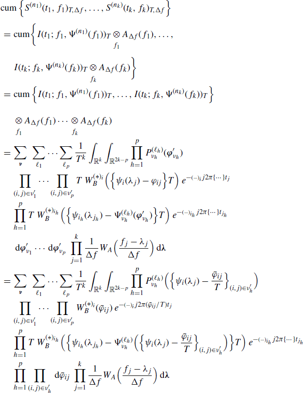
By substituting the STFT expression (4.94b) and (4.107) (with Δf = 1/T) into the cross-periodogram definition we formally have

(5.128)

Thus, let

(5.129)

for the multilinearity property of cumulants (Mendel 1991) we have

(5.130)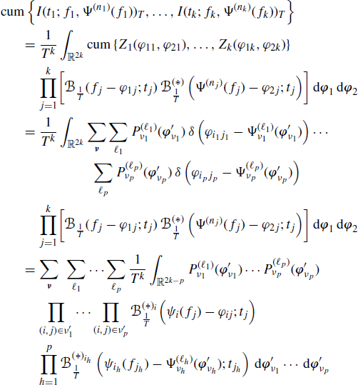

where, ϕ₁ [ϕ₁₁, …, ϕ_1k], ϕ₂ [ϕ₂₁, …, ϕ_2k], . In the second equality (5.124) and (5.126) are accounted for; in the third equality the sampling property of Dirac delta is used and here and in the following (*)_i = (*) if i = 1 and (*)_i = (*) * if i = 2.

Using again the multilinearity property of cumulants (Mendel 1991), the result is that

(5.131)

where, in the third equality Assumptions 4.4.5 (data-tapering window regularity) (with Δf = 1/T) and 4.6.2 (frequency-smoothing window regularity) are accounted for; and in the fourth equality the variable changes

are made in the inner integrals in (with λ fixed) so that, according to notation introduced in (5.127), the result is that

Starting from the bounds derived in (5.133) and (5.138), the interchange of the order of cum, expectation, and integral operations can be justified by the Fubini and Tonelli theorem (Champeney 1990, Chapter 3). Furthermore, the same bounds justify the interchange of infinite sums and integral operations by the Weierstrass criterion (Smirnov 1964).

Let us consider the only term corresponding to the only partition with p = 1 in (5.131). The set ν₁ is coincident with the whole rectangular k × 2 table and with (i₁, j₁) = (2, k).

(5.132)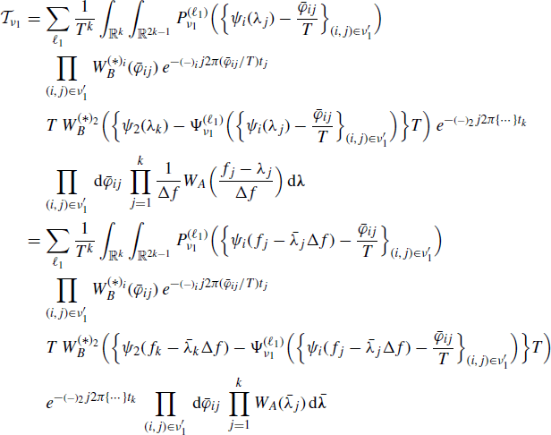

where and in the second equality the variable change

(so that ) is made.

Accounting for Assumptions 4.4.5 (data-tapering window regularity), 4.6.2 (frequency-smoothing window regularity), 4.7.8 (spectral cumulants), it results in

(5.133)

Therefore,

(5.134)

and, hence,

(5.135)

The k × 2 table (5.123) has two columns and partitions are indecomposable (see comments following Assumption 2.4.15). Thus, for p ≥ 2 each set ν_m hooks with one or two other sets of the partition. Specifically, two sets (those containing at least one element of the first row or at least one element of the last row) hook with one set and the remaining p − 2 sets hook with two sets. Consequently, for p ≥ 2, each set ν_m has at least one line containing only one pair of indices. Let us choose as pair (i_m, j_m) in Fact 5.6.1 the pair of indices corresponding to the lower of these lines of ν_m containing only one pair. Thus j_m is a row index not shared with any other pair , where is obtained by ν_m by removing the element (i_m, j_m). The case is different for the only partition containing only one element (p = 1). In such a case, j_m = k is a row index shared by (i_m, j_m) = (2, k) with the element (1, k).

Let us consider now the generic term with p > 1 in (1.131).

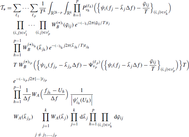
Since p ≥ 2 and sets ν_h hook, we can select (i_h, j_h) so that no other pair has j = j_h. Moreover, there are p − 1 distinct indices j_h and j_p = j_p−1. Let us interchange the order of integrals

and let us make the variable changes

Then, for h = 1, …, p − 1, order the integrals so that the innermost is that in and make the variable change

( fixed). Since no other pair has j = j_h, then

(5.136)

Thus,

(5.137)

where

Let denote the inverse function of . It follows that is bounded due to Assumption 4.7.9. Thus,

(5.138)

That is,

(5.139)

with 2 ≤ p ≤ 2k. Hence

(5.140)

For k = 2 from (5.140), we have

(5.141)

The above limit is bounded for all partitions ν with k = 2 only if the processes are zero mean. In fact, in such a case terms with p = 3 and p = 4 are identically zero (only terms with p = 1 and p = 2 are nonzero, see (5.11)). For k = 2 and zero-mean processes a tighter bound is provided by Theorems 4.7.7 and 5.8.2, for which

(5.142)

For k ≥ 3 from (5.140) we have

(5.143)

provided that the order of the two limits is not interchanged. In fact, for Δf finite, the limit as T→ ∞ is zero for k ≥ 3. In contrast, for T finite, since 2 ≤ p ≤ 2k, the limit as Δf → 0 is infinite for those partitions ν with p ≥ k/2 + 1.

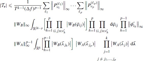
The interchange of the order of integrals in the expression of to obtain (5.137) is justified by the Fubini and Tonelli theorem (Champeney 1990, Chapter 3). In fact, let be T^k−1(Δf)^p−1 times the integrand function in the expression of in (5.137). One has

(5.144)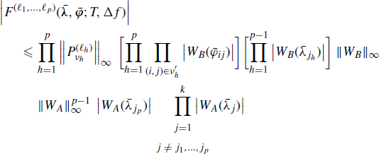

with the rhs belonging to due to Assumptions 4.4.5 (data-tapering window regularity) and 4.6.2 (frequency-smoothing window regularity).

5.6.2 Proof of Theorem 4.7.11 Asymptotic Joint Complex Normality of the Frequency-Smoothed Cross-Periodograms

From Theorem 4.7.6 it follows that

(5.145)

The rate of decay to zero of Δf should be such that approaches zero as T→ ∞ and Δf → 0 with TΔf→ ∞. Let us assume that

(5.146)

with 0 < a < 1. Then, as T→ ∞, Δf_T = T^−a → 0 with TΔf_T = T^1−a→ ∞. In addition, we have

(5.147)

Consequently, approaches zero as T→ ∞ provided that

(5.148)

Therefore, the condition on a is

(5.149)

From Theorem 4.7.7 it follows that the asymptotic covariance

(5.150)

is finite. Analogously, from Theorem 5.8.3 it follows that the asymptotic conjugate covariance is finite. Moreover, from Lemma 4.7.10 with k ≥ 3 we have

(5.151)

Since the value of the cumulant does not change by adding a constant to each of the random variables (Brillinger 1981, Theorem 2.3.1), we also have

(5.152)

That is, for every fixed n_i, f_i, t_i, the random variables

i = 1, …, k, are asymptotically (T→ ∞ and Δf → 0 with TΔf→ ∞) zero-mean jointly complex Normal (Section 1.4.2).