
7.4 Constant Relative Radial Acceleration
According to notation introduced in Section 7.3, we have
(7.193) ![]()
(7.195) ![]()
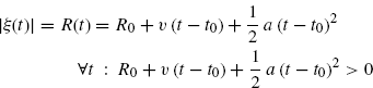
Let us assume that the relative radial acceleration between P T(t − D(t)) and P R(t) is constant within the observation interval, that is,
(7.196) ![]()
then
where ![]() and ξ0 = ξ(t0).
and ξ0 = ξ(t0).
Note that motion with constant acceleration is not compatible with the special relativity theory. In fact, from (7.197) it follows that
(7.199) ![]()
Consequently, such a motion model can be used provided that the length T of the observation interval is not too large.
Let us assume that TX and RX do not collapse within the observation interval. Then, from (7.194) and (7.198) we have
where the upper sign is for ξ(t) ≥ 0 and the lower is for ξ(t) < 0. That is, D(t) depends quadratically on t:
with ![]() ,
, ![]() , d2 = ± aξ/(2c).
, d2 = ± aξ/(2c).
7.4.1 Stationary TX, Moving RX
In the case of stationary TX and moving RX, (7.11) specializes into (7.34) and (7.35). Assuming that during the observation interval RX does not collapse on TX, we have
From (7.198), (7.202), and (7.203), it follows
and comparing (7.198) and (7.204) it results in ![]() , a = aξ for ξ(t) ≥ 0 and
, a = aξ for ξ(t) ≥ 0 and ![]() , a = − aξ for ξ(t) < 0. In addition, (7.203) and (7.204) lead to
, a = − aξ for ξ(t) < 0. In addition, (7.203) and (7.204) lead to
(7.205) ![]()
That is, the time-varying delay depends quadratically on t and in (7.201) one has ![]() ,
, ![]() , d2 = a/(2c).
, d2 = a/(2c).
7.4.2 Moving TX, Stationary RX
In the case of moving TX and stationary RX, (7.11) specializes into (7.37) and (7.38). Assuming that during the observation interval TX does not collapse on RX, we have
From (7.198) and (7.206) it follows
where the upper sign is for ξ(t) ≥ 0 and the lower for ξ(t) < 0. As in the case of stationary TX and moving RX, D(t) depends quadratically on t. The time behavior of R(t) cannot be easily derived using (7.207) with (7.208) substituted into.