Chapter 5
Design Considerations of Primary Systems
Imagination is more important than knowledge.
Albert Einstein
The great end of learning is nothing else but to seek for the lost mind.
Mencius, Works, 299 BC
Earn your ignorance! Learn something about everything before you know nothing about anything.
Turan Gönen
5.1 Introduction
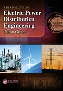
The part of the electric utility system that is between the distribution substation and the distribution transformers is called the primary system. It is made of circuits known as primary feeders or primary distribution feeders.
Figure 5.1 shows a one-line diagram of a typical primary distribution feeder. A feeder includes a “main” or main feeder, which usually is a three-phase four-wire circuit, and branches or laterals, which usually are single-phase or three-phase circuits tapped off the main. Also sublaterals may be tapped off the laterals as necessary. In general, laterals and sublaterals located in residential and rural areas are single phase and consist of one-phase conductor and the neutral. The majority of the distribution transformers are single phase and are connected between the phase and the neutral through fuse cutouts.
One-line diagram of typical primary distribution feeders.
(From Fink, D.G. and Beaty, H.W., Standard Handbook for Electrical Engineers, 11th edn., McGraw-Hill, New York, 1978.)
A given feeder is sectionalized by reclosing devices at various locations in such a manner as to remove the faulted circuit as little as possible so as to hinder service to as few consumers as possible. This can be achieved through the coordination of the operation of all the fuses and reclosers.
It appears that, due to growing emphasis on the service reliability, the protection schemes in the future will be more sophisticated and complex, ranging from manually operated devices to remotely controlled automatic devices based on supervisory controlled or computer-controlled systems.
The congested and heavy-load locations in metropolitan areas are served by using underground primary feeders. They are usually radial three-conductor cables. The improved appearance and less frequent trouble expectancy are among the advantages of this method. However, it is more expensive, and the repair time is longer than the overhead systems. In some cases, the cable can be employed as suspended on poles. The cost involved is greater than that of open wire but much less than that of underground installation. There are various and yet interrelated factors affecting the selection of a primary-feeder rating. Examples are
- The nature of the load connected
- The load density of the area served
- The growth rate of the load
- The need for providing spare capacity for emergency operations
- The type and cost of circuit construction employed
- The design and capacity of the substation involved
- The type of regulating equipment used
- The quality of service required
- The continuity of service required
The voltage conditions on distribution systems can be improved by using shunt capacitors that are connected as near the loads as possible to derive the greatest benefit. The use of shunt capacitors also improves the power factor involved, which in turn lessens the voltage drops and currents, and therefore losses, in the portions of a distribution system between the capacitors and the bulk power buses. The capacitor ratings should be selected carefully to prevent the occurrence of excessive overvoltages at times of light loads due to the voltage rise produced by the capacitor currents.
The voltage conditions on distribution systems can also be improved by using series capacitors. But the application of series capacitors does not reduce the currents and therefore losses, in the system.
5.2 Radial-Type Primary Feeder
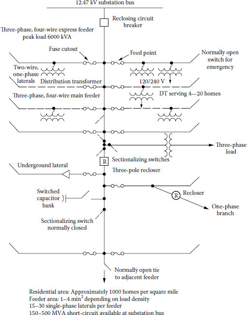
The simplest and the lowest cost and therefore the most common form of primary feeder is the radial-type primary feeder as shown in Figure 5.2. The main primary feeder branches into various primary laterals that in turn separates into several sublaterals to serve all the distribution transformers. In general, the main feeder and subfeeders are three-phase three- or four-wire circuits and the laterals are three phase or single phase. The current magnitude is the greatest in the circuit conductors that leave the substation. The current magnitude continually lessens out toward the end of the feeder as laterals and sublaterals are tapped off the feeder. Usually, as the current lessens, the size of the feeder conductors is also reduced. However, the permissible voltage regulation may restrict any feeder size reduction, which is based only on the thermal capability, that is, current-carrying capacity, of the feeder.
The reliability of service continuity of the radial primary feeders is low. A fault occurrence at any location on the radial primary feeder causes a power outage for every consumer on the feeder unless the fault can be isolated from the source by a disconnecting device such as a fuse, sectionalizer, disconnect switch, or recloser.
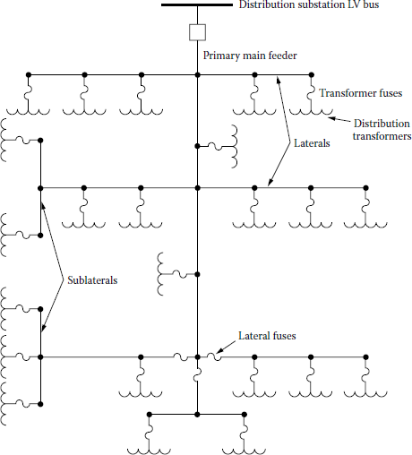
Figure 5.3 shows a modified radial-type primary feeder with tie and sectionalizing switches to provide fast restoration of service to customers by switching unfaulted sections of the feeder to an adjacent primary feeder or feeders. The fault can be isolated by opening the associated disconnecting devices on each side of the faulted section.
Figure 5.4 shows another type of radial primary feeder with express feeder and backfeed. The section of the feeder between the substation low-voltage bus and the load center of the service area is called an express feeder. No subfeeders or laterals are allowed to be tapped off the express feeder. However, a subfeeder is allowed to provide a backfeed toward the substation from the load center.
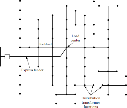
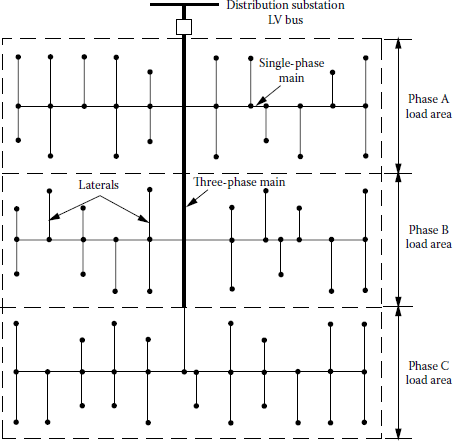
Figure 5.5 shows a radial-type phase-area feeder arrangement in which each phase of the threephase feeder serves its own service area. In Figures 5.4 and 5.5, each dot represents a balanced three-phase load lumped at that location.
5.3 Loop-Type Primary Feeder
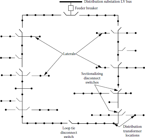
Figure 5.6 shows a loop-type primary feeder that loops through the feeder load area and returns back to the bus. Sometimes the loop tie disconnect switch is replaced by a loop tie breaker due to the load conditions. In either case, the loop can function with the tie disconnect switches or breakers normally open (NO) or normally closed.
Usually, the size of the feeder conductor is kept the same throughout the loop. It is selected to carry its normal load plus the load of the other half of the loop. This arrangement provides two parallel paths from the substation to the load when the loop is operated with NO tie breakers or disconnect switches.
A primary fault causes the feeder breaker to be open. The breaker will remain open until the fault is isolated from both directions. The loop-type primary-feeder arrangement is especially beneficial to provide service for loads where high service reliability is important. In general, a separate feeder breaker on each end of the loop is preferred, despite the cost involved. The parallel feeder paths can also be connected to separate bus sections in the substation and supplied from separate transformers. In addition to main feeder loops, NO lateral loops are also used, particularly in underground systems.
5.4 Primary Network
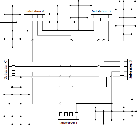
As shown in Figure 5.7, a primary network is a system of interconnected feeders supplied by a number of substations. The radial primary feeders can be tapped off the interconnecting tie feeders. They can also be served directly from the substations. Each tie feeder has two associated circuit breakers at each end in order to have less load interrupted due to a tie-feeder fault.
The primary-network system supplies a load from several directions. Proper location of transformers to heavy-load centers and regulation of the feeders at the substation buses provide for adequate voltage at utilization points. In general, the losses in a primary network are lower than those in a comparable radial system due to load division.
The reliability and the quality of service of the primary-network arrangement are much higher than the radial and loop arrangements. However, it is more difficult to design and operate than the radial or loop systems.
5.5 Primary-Feeder Voltage Levels
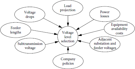
The primary-feeder voltage level is the most important factor affecting the system design, cost, and operation. Some of the design and operation aspects affected by the primary-feeder voltage level are [2]
- Primary-feeder length
- Primary-feeder loading
- Number of distribution substations
- Rating of distribution substations
- Number of subtransmission lines
- Number of customers affected by a specific outage
- System maintenance practices
- The extent of tree trimming
- Joint use of utility poles
- Type of pole-line design and construction
- Appearance of the pole line
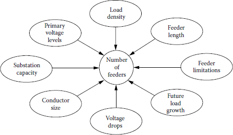
There are additional factors affecting the decisions for primary-feeder voltage-level selection, as shown in Figure 5.8. Table 5.1 gives typical primary voltage levels used in the United States. Three-phase four-wire multigrounded common neutral primary systems, for example, 12.47Y/7.2 kV, 24.9Y/14.4 kV, and 34.5Y/19.92 kV, are employed almost exclusively. The fourth wire is used as the multigrounded neutral for both the primary and secondary systems. The 15 kV-class primary voltage levels are most commonly used. The most common primary distribution voltage in use throughout North America is 12.47 kV. However, the current trend is toward higher voltages, for example, the 34.5 kV class is gaining rapid acceptance. The 5 kV class continues to decline in usage. Some distribution systems use more than one primary voltage, for example, 12.47 and 34.5 kV. California is one of the few states that has three-phase three-wire primary systems. The four-wire system is economical, especially for underground residential distribution (URD) systems, since each primary lateral has only one insulated phase wire and the bare neutral instead of having two insulated wires.
Typical Primary Voltage Levels
Class, kV |
3φ Voltage | |
|---|---|---|
2.5 |
2,300 |
3W-Δ |
2,400a |
3W-Δ |
|
5.0 |
4,000 |
3W-Δ or 3W-Y |
4,160a |
4W-Y |
|
4,330 |
3W-Δ |
|
4,400 |
3W-Δ |
|
4,600 |
3W-Δ |
|
4,800 |
3W-Δ |
|
8.66 |
6,600 |
3W-Δ |
6,900 |
3W-Δ or 4W-Y |
|
7,200a |
3W-Δ or 4W-Y |
|
7,500 |
4W-Y |
|
8,320 |
4W-Y |
|
15 |
11,000 |
3W-Δ |
11,500 |
3W-Δ |
|
12,000 |
3W-Δ or 4W-Y |
|
12,470a |
4W-Y |
|
13,200a |
3W-Δ or 4W-Y |
|
13,800a |
3W-Δ |
|
14,400 |
3W-Δ |
|
25 |
22,900a |
4W-Y |
24,940a |
4W-Y |
|
34.5 |
34,500a |
4W-Y |
a Most common voltage in the individual classes.
Usually, primary feeders located in low-load density areas are restricted in length and loading by permissible voltage drop rather than by thermal restrictions, whereas primary feeders located in high-load density areas, for example, industrial and commercial areas, may be restricted by thermal limitations.
In general, for a given percent voltage drop, the feeder length and loading are direct functions of the feeder voltage level. This relationship is known as the voltage-square rule. For example, if the feeder voltage is doubled, for the same percent voltage drop, it can supply the same power four times the distance. However, as Lokay [2] explains it clearly, the feeder with the increased length feeds more load. Therefore, the advantage obtained by the new and higher-voltage level through the voltage-square factor, that is,
Voltage-square factor = (VL−N,newVL−N,old)2 (5.1)
has to be allocated between the growth in load and in distance. Further, the same percent voltage drop will always result provided that the following relationship exists:
Distance ratio×Load ratio= Voltage-square factor (5.2)
where
Distance ratio=NewdistanceOld distance (5.3)
and
Load ratio=Newfeeder loadingOld feeder loading (5.4)
The relationship between the voltage-square factor rule and the feeder distance-coverage principle is further explained in Figure 5.9.
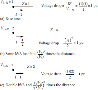
Illustration of the voltage-square rule and the feeder distance-coverage principle as a function of feeder voltage level and a single load.
(From Westinghouse Electric Corporation, Electric Utility Engineering Reference Book-Distribution Systems, Vol. 3, East Pittsburgh, Pittsburgh, PA, 1965.)
There is a relationship between the area served by a substation and the voltage rule. Lokay [2] defines it as the area-coverage principle. As illustrated in Figure 5.10, for a constant percent voltage drop and a uniformly distributed load, the feeder service area is proportional to
[(VL−N,newVL−N,old)2]2/3(5.5)
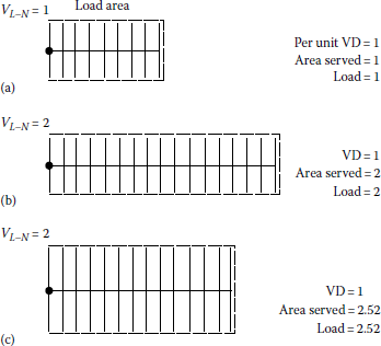
Feeder area-coverage principle as related to feeder voltage and a uniformly distributed load.
(From Westinghouse Electric Corporation, Electric Utility Engineering Reference Book-Distribution Systems, Vol. 3, East Pittsburgh, Pittsburgh, PA, 1965.)
provided that both dimensions of the feeder service area change by the same proportion. For example, if the new feeder voltage level is increased to twice the previous voltage level, the new load and area that can be served with the same percent voltage drop are
[(VL−N,newVL−N,old)2]2/3=(22)2/3=2.52 (5.6)
times the original load and area. If the new feeder voltage level is increased to three times the previous voltage level, the new load and area that can be served with the same percent voltage drop are times the original load and area.
[(VL−N,newVL−N,old)2]2/3 =(32)2/3=4.32 (5.7)
5.6 Primary-Feeder Loading
Primary-feeder loading is defined as the loading of a feeder during peak-load conditions as measured at the substation [2]. Some of the factors affecting the design loading of a feeder are
- The density of the feeder load
- The nature of the feeder load
- The growth rate of the feeder load
- The reserve-capacity requirements for emergency
- The service-continuity requirements
- The service-reliability requirements
- The quality of service
- The primary-feeder voltage level
- The type and cost of construction
- The location and capacity of the distribution substation
- The voltage regulation requirements
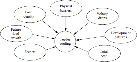
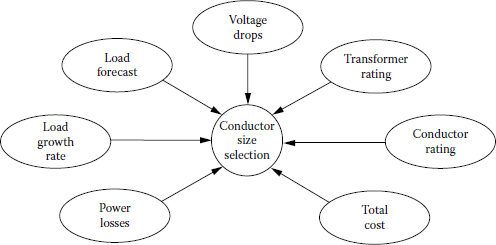
There are additional factors affecting the decisions for feeder routing, the number of feeders, and feeder conductor size selection, as shown in Figures 5.11 through 5.13.
5.7 Tie Lines
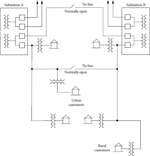
A tie line is a line that connects two supply systems to provide emergency service to one system from another, as shown in Figure 5.14. Usually, a tie line provides service for area loads along its route as well as providing for emergency service to adjacent areas or substations. Therefore, tie lines are needed to perform either of the following two functions:
- To provide emergency service for an adjacent feeder for the reduction of outage time to the customers during emergency conditions.
- To provide emergency service for adjacent substation systems, thereby eliminating the necessity of having an emergency backup supply at every substation. Tie lines should be installed when more than one substation is required to serve the area load at one primary distribution voltage.
Usually the substation primary feeders are designed and installed in such an arrangement as to have the feeders supplied from the same transformer extend in opposite directions so that all required ties can be made with circuits supplied from different transformers. For example, a substation with two transformers and four feeders might have the two feeders from one transformer extending north and south. The two feeders from the other transformer may extend east and west. All tie lines should be made to circuits supplied by other transformers. This would make it much easier to restore service to an area that is affected by a transformer failure.
Disconnect switches are installed at certain intervals in main feeder tie lines to facilitate load transfer and service restoration. The location of disconnect switches needs to be selected carefully to obtain maximum operating flexibility. Not only the physical arrangement of the circuit but also the size and nature of loads between switches are important. Loads between the disconnect switches should be balanced as much as possible so that load transfers between circuits do not adversely affect circuit operation. The optimum voltage conditions are obtained only if the circuit is balanced as closely as possible throughout its length.
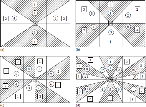
5.8 Distribution Feeder Exit: Rectangular-Type Development
The objective of this section is to provide an example for a uniform area development plan to minimize the circuitry changes associated with the systematic expansion of the distribution system.
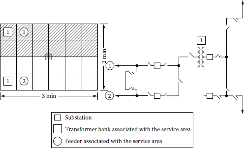
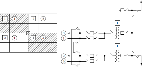
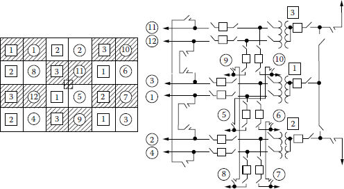
Assume that underground feeder exits are extended out of a distribution substation into an existing overhead system. Also assume that at the ultimate development of this substation, a 6 min2 service area will be served with a total of 12 feeder circuits, four per transformer. Assuming uniform load distribution, each of the 12 circuits would serve approximately ½ mi2 in a fully developed service area. This is called the rectangular-type development and illustrated in Figures 5.15 through 5.18.
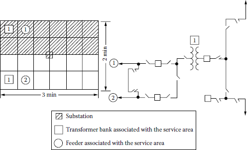
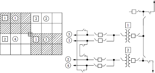
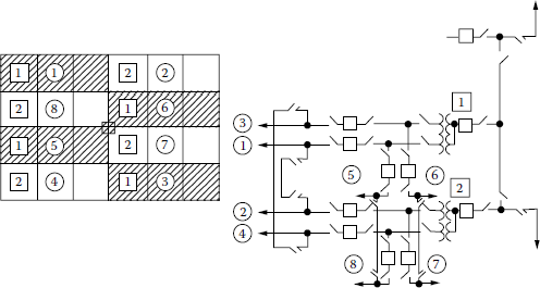
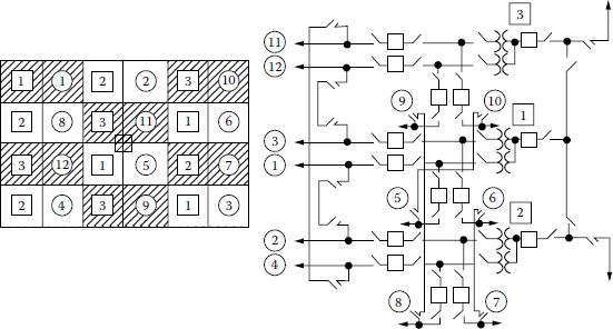
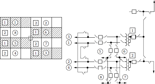
In general, adjacent service areas are served from different transformer banks in order to provide for transfer to adjacent circuits in the event of transformer outages. The addition of new feeder circuits and transformer banks requires circuit number changes as the service area develops. The center transformer bank is always fully developed when the substation has eight feeder circuits. As the service area develops, the remaining transformer banks develop to full capacity. There are two basic methods of development, depending upon the load density of a service area, namely, the 1-2-4-8-12 feeder circuit method and the 1-2-4-6-8-12 feeder circuit method. The numbers shown for feeders and transformer banks in the following figures represent only the sequence of installation as the substation develops.
Method of development for high-load density areas: In service areas with high-load density, the adjacent substations are developed similarly to provide for adequate load-transfer capability and service continuity. Here, for example, a two-transformer-bank substation can carry a firm rating of the emergency rating of one bank plus circuit ties, plus reserve considerations. Since sufficient circuit ties must be available to support the loss of a large transformer unit, the 1-2-4-8-12 feeder method is especially desirable for a high-load density area. Figures 5.15 through 5.18 show the sequence of installing additional transformers and feeders.
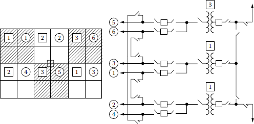
Method of development for low-load density areas: In low-load density areas, where adjacent substations are not adequately developed and circuit ties are not available due to excessive distances between substations, the 1-2-4-6-8-12 circuit-developing substation scheme is more suitable. These large distances between substations generally limit the amount of load that can be transferred between substations without objectionable outage time due to circuit switching and guarantee that minimum voltage levels are maintained. This method requires the substation to have all three transformer banks before using the larger transformers in order to provide a greater firming capability within the individual substation.
As illustrated in Figures 5.19 through 5.23, once three, for example, 12/16/20-MVA, transformer units and six feeders are reached in the development of this type of substation, there are two alternatives for further expansion: (1) either remove one of the banks and increase the remaining two bank sizes to the larger, for example, 24/32/40 MVA, transformer units employing the low-side bays of the third transformer as part of the circuitry in the development of the remaining two banks, or (2) completely ignore the third transformer-bank area and complete the development of two remaining sections similar to the previous method.
5.9 Radial-Type Development
In addition to the rectangular-type development associated with overhead expansion, there is a second type of development that is due to the growth of URD subdivisions with underground feeders serving local load as they exit into the adjacent service areas. At these locations, the overhead feeders along the quarter section lines are replaced with underground cables, and as these underground lines extend outward from the substation, the area load is served. These underground lines extend through the platted service area developments and terminate usually on a remote overhead feeder along a section line. This type of development is called radial-type development, and it resembles a wagon wheel with the substation as the hub and the radial spokes as the feeders, as shown in Figure 5.24.
5.10 Radial Feeders with Uniformly Distributed Load
The single-line diagram, shown in Figure 5.25, illustrates a three-phase feeder main having the same construction, that is, in terms of cable size or open-wire size and spacing, along its entire length l. Here, the line impedance is z = r + jx per unit length.
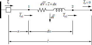
The load flow in the main is assumed to be perfectly balanced and uniformly distributed at all locations along the main. In practice, a reasonably good phase balance sometimes is realized when single-phase and open-wye laterals are wisely distributed among the three phases of the main.
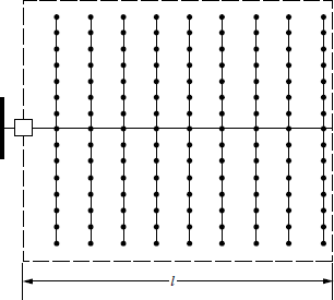
Assume that there are many closely spaced loads and/or lateral lines connected to the main but not shown in Figure 5.25. Since the load is uniformly distributed along the main, as shown in Figure 5.26, the load current in the main is a function of the distance. Therefore, in view of the many closely spaced small loads, a differential tapped-off load current dĪ, which corresponds to a dx differential distance, is to be used as an idealization. Here, l is the total length of the feeder and x is the distance of the point 1 on the feeder from the beginning end of the feeder. Therefore, the distance of point 2 on the feeder from the beginning end of the feeder is x + dx. Īs is the sending-end current at the feeder breaker, and Īr is the receiving-end current. Īx1 and Īx2 are the currents in the main at points 1 and 2, respectively. Assume that all loads connected to the feeder have the same power factor.
The following equations are valid both in per-unit or per-phase (line-to-neutral) dimensional variables. The circuit voltage is of either primary or secondary, and therefore shunt capacitance currents may be neglected. Since the total load is uniformly distributed from x = 0 to x = ℓ,
dˉIdx= ˉk (5.8)
which is a constant. Therefore Īx, that is, the current in the main of some x distance away from the circuit breaker, can be found as a function of the sending-end current Īs and the distance x. This can be accomplished either by inspection or by writing a current equation containing the integration of dĪ. Therefore, for dx distance,
ˉIx1=ˉIx2+dˉI (5.9)
or
ˉIx2=ˉIx1−dˉI (5.10)
From Equation 5.10,
ˉIx2=ˉIx1−dˉIdxdx=ˉIx1−dˉIdxdx(5.11)
or
ˉIx2=ˉIx1−ˉkdx (5.12)
where ˉk= dĪ/dx or, approximately,
ˉIx2=ˉIx1−kdˉI (5.13)
and
ˉIx1=ˉIx2+kdˉI (5.14)
Therefore, for the total feeder,
Ir=Is−k×l (5.15)
and
Is=Ir+k×l (5.16)
When x = l, from Equation 5.15,
Ir=Is−k×l=0
hence
k=Isl (5.17)
and since x = l,
Ir=Is−k×x (5.18)
Therefore, substituting Equation 5.17 into Equation 5.18,
Ir=Is(1−xl) (5.19)
For a given x distance,
Ix=Ir
thus Equation 5.19 can be written as
Ix=Is(1−xl) (5.20)
which gives the current in the main at some x distance away from the circuit breaker. Note that from Equation 5.20,
Is={Ir=0at x=lIr=Isat x=0
The differential series voltage drop dˉVand the differential power loss dPLS due to I2R losses can also be found as a function of the sending-end current Is and the distance x in a similar manner. Therefore, the differential series voltage drop can be found as
dˉV=Ix×zdx (5.21)
or substituting Equation 5.20 into Equation 5.21,
dˉV=Is×z(1−xl)dx (5.22)
Also, the differential power loss can be found as
dPLS=I2x×rdx (5.23)
or substituting Equation 5.20 into Equation 5.23,
dPLS=[Is(1−xl)]2rdx (5.24)
The series voltage drop VDx due to Ix current at any point x on the feeder is
VDx=x∫0dV (5.25)
Substituting Equation 5.22 into Equation 5.25,
VDx=∫0Is×z(1−xl)dx (5.26)
or
VDx=Is×z×x(1−x2l) (5.27)
Therefore, the total series voltage drop ∑VDxon the main feeder when x = l is
∑VDx=Is×z×l(1−l2l)
or
∑VDx=12z×l×Is (5.28)
The total copper loss per phase in the main due to I2R losses is
∑PLS=l∫0dPLS (5.29)
or
∑PLS=13I2s×r×l (5.30)
Therefore, from Equation 5.28, the distance x from the beginning of the main feeder at which location the total load current Is may be concentrated, that is, lumped for the purpose of calculating the total voltage drop, is
x=l2
whereas, from Equation 5.30, the distance x from the beginning of the main feeder at which location the total load current Is may be lumped for the purpose of calculating the total power loss is
x=l3
5.11 Radial Feeders with Nonuniformly Distributed Load
The single-line diagram, shown in Figure 5.27, illustrates a three-phase feeder main, which has the tapped-off load increasing linearly with the distance x. Note that the load is zero when x = 0. The plot of the sending-end current vs. the x distance along the feeder main gives the curve shown in Figure 5.28.
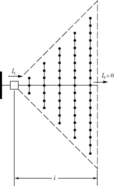
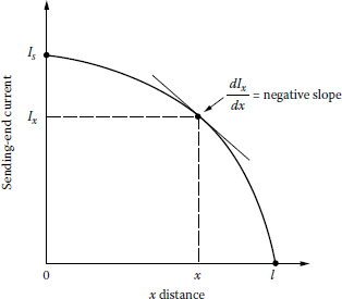
From Figure 5.28, the negative slope can be written as
dIxdx=−k×Is×x (5.31)
Here, the constant k can be found from
Is=l∫x=0−dIx=l∫x=0k×Is×xdx(5.32)
or
Is=k×Is×l22 (5.33)
From Equation 5.33, the constant k is
k=2l2 (5.34)
Substituting Equation 5.34 into Equation 5.31,
dIxdx=−2Is×xl2 (5.35)
Therefore, the current in the main at some x distance away from the circuit breaker found as
Ix=Is(1−x2l2) (5.36)
Hence, the differential series voltage drop is
dˉV=Ix×zdx (5.37)
or
dˉV=Is×z(1−x2l2)dx (5.38)
Also, the differential power loss can be found as
dPLS=I2x×rdx (5.39)
or
dPLS=I2s×r(1−x2l2)dx (5.40)
The series voltage drop due to Ix current at any point x on the feeder is
VDx=x∫0dV (5.41)
Substituting Equation 5.38 into Equation 5.41 and integrating the result,
VDx=Is×z×x(1−x23l2) (5.42)
Therefore, the total series voltage drop on the main feeder when x = 1 is
∑VDx=23z×l×Is (5.43)
The total copper loss per phase in the main due to I2R losses is
∑PLS=l∫0dPLS (5.44)
or
∑PLS=815I2s×r×l (5.45)
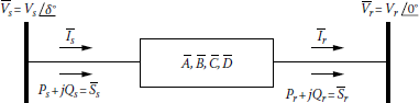
5.12 Application of the A, B, C, D General Circuit Constants to Radial Feeders
Assume a single-phase or balanced three-phase transmission or distribution circuit characterized by the ¯A, ¯B, ¯C, ˉDgeneral circuit constants, as shown in Figure 5.29. The mixed data assumed to be known, as commonly encountered in system design, are |ˉVS| , Pr, and cos θ. Assume that all data represent either per-phase dimensional values or per unit values.
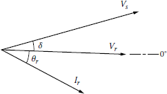
As shown in Figure 5.30, taking phasor ˉVras the reference,
ˉVr=Vr∠0°(5.46)
ˉV=sVs∠δ(5.47)
ˉIr=Ir∠−θr (5.48)
where
ˉVr= receiving-end voltage phasor
ˉVs= sending-end voltage phasor
ˉIr= receiving-end current phasor
The sending-end voltage in terms of the general circuit constants can be expressed as
ˉVs=ˉA×ˉVr+ˉB×ˉIr (5.49)
where
ˉA=ˉA1+jˉA2 (5.50)
ˉB=ˉB1+jˉB2 (5.51)
ˉIr=Ir(cosθr−jsinθr) (5.52)
ˉVr=Vr∠0°=Vr (5.53)
ˉVs=Vs(cosδ+jsinδ) (5.54)
Therefore, Equation 5.49 can be written as
Vscosδ+jVssinδ=(A1+jA2)Vr+(B1+jB2)(Ircosθr−jIrsinθr)
from which
Vscosδ=A1Vr+B1Ircosθr+B2Irsinθr (5.55)
and
Vssinδ=A2Vr+B2Ircosθr−B1Irsinθr (5.56)
By taking squares of Equations 5.55 and 5.56, and adding them side by side,
V2s=(A1Vr+B1Ircosθr+B2Irsinθr)2+(A2Vr+B2Ircosθr−B1Irsinθr)2 (5.57)
or
V2s=V2s(A21+A22)+2VrIrcosθr(A1B1+A2B2)+B21(V2rcos2θr+I2rsin2θr)+B22(I2rsin2θr+I2rcos2θr)+2VrIrsinθr(A1B2−B1A2) (5.58)
Since
Pr=VrIrcosθr (5.59)
Qr=VrIrsinθr (5.60)
and
Qr=Prtanθ (5.61)
Equation 5.58 can be rewritten as
V2r(A21+A22)+(B21+B22)(1+tan2θr)P2rV2r=V2s−2Pr[(A1B1+A2B2)+(A1B2−B1A2)tanθr] (5.62)
Let
Then Equation 8.62 becomes
or
Therefore, from Equation 5.65, the receiving-end voltage can be found as
Also, from Equations 5.55 and 5.56,
and
where
Therefore,
and
By dividing Equation 5.68 by Equation 5.69,
or
Equations 5.66 and 5.71 are found for a general transmission system. They could be adapted to the simpler transmission consisting of a short primary-voltage feeder where the feeder capacitance is usually negligible, as shown in Figure 5.31.
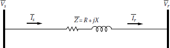
To achieve the adaptation, Equations 5.63, 5.66, and 5.71 can be written in terms of R and X. Therefore, for the feeder shown in Figure 5.31,
or
where
Therefore,
or
where
and
Similarly,
or
where
and
Substituting Equations 5.79, 5.80, 5.83, and 5.84 into Equation 5.66,
or
or
where
Also, from Equation 5.71,
Example 5.1
Assume that the radial express feeder, shown in Figure 5.31, is used on rural distribution and is connected to a lumped-sum (or concentrated) load at the receiving end. Assume that the feeder impedance is 0.10 + j0.10 pu, the sending-end voltage is 1.0 pu, Pr is 1.0 pu constant power load, and the power factor at the receiving end is 0.80 lagging. Use the given data and the exact equations for K, Pr, and tan δ given previously and determine the following:
- Compute Vr and δ by using the exact equations and find also the corresponding values of the Ir and Is currents.
- Verify the numerical results found in part (a) by using those results in
Solution
- From Equation 5.88,
From Equation 5.87,
From Equation 5.89,
therefore
- From the given equation,
5.13 Design of Radial Primary Distribution Systems
The radial primary distribution systems are designed in several different ways: (1) overhead primaries with overhead laterals or (2) URD, for example, with mixed distribution of overhead primaries and underground laterals.
5.13.1 Overhead Primaries
For the sake of illustration, Figure 5.32 shows an arrangement for overhead distribution, which includes a main feeder and 10 laterals connected to the main with sectionalizing fuses. Assume that the distribution substation, shown in the figure, is arbitrarily located; it may also serve a second area, which is not shown in the figure, that is equal to the area being considered and, for example, located “below” the shown substation site.
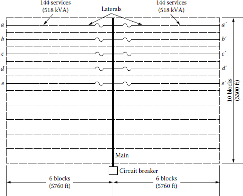
Here, the feeder mains are three phase and of 10 short block length or less. The laterals, on the other hand, are all of six long block length and are protected with sectionalizing fuses. In general, the laterals may be either single phase, open wye grounded, or three phase.
Here, in the event of a permanent fault on a lateral line, only a relatively small fraction of the total area is outaged. Ordinarily, permanent faults on the overhead line can be found and repaired quickly.
5.13.2 Underground Residential Distribution
Even though a URD costs somewhere between 1.25 and 10 times more than a comparable overhead system, due to its certain advantages, it is used commonly [4,5]. Among the advantages of the underground system are the following:
- The lack of outages caused by the abnormal weather conditions such as ice, sleet, snow, severe rain and storms, and lightning
- The lack of outages caused by accidents, fires, and foreign objects
- The lack of tree trimming and other preventative maintenance tasks
- The aesthetic improvement
For the sake of illustration, Figure 5.33 shows a URD for a typical overhead and underground primary distribution system of the two-way feed type. The two arbitrarily located substations are assumed to be supplied from the same subtransmission line, which is not shown in the figure, so that the low-voltage buses of the two substations are nominally in phase. In the figure, the two overhead primary-feeder mains carry the total load of the area being considered, that is, the area of the 12 block by 10 block. The other two overhead feeder mains carry the other equally large area. Therefore, in this example, each area has 120 blocks.
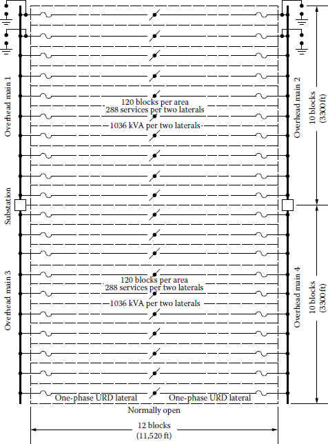
The laterals, in residential areas, typically are single phase and consist of directly buried (rather than located in ducts) concentric neutral-type cross-linked polyethylene (XLPE)-insulated cable. Such cables usually insulated for 15 kV line-to-line solidly grounded neutral service and the commonly used single-phase line-to-neutral operating voltages are nominally 7200 or 7620 V.
The installation of long lengths of cable capable of being plowed directly into the ground or placed in narrow and shallow trenches, without the need for ducts and manholes, naturally reduces installation and maintenance costs. The heavy three-phase feeders are overhead along the periphery of a residential development, and the laterals to the pad-mount transformers are buried about 40 in. deep. The secondary service lines then run to the individual dwellings at a depth of about 24 in. and come up into the dwelling meter through a conduit. The service conductors run along easements and do not cross adjacent property lines.
The distribution transformers now often used are of the pad-mounted or submersible type. The pad-mounted distribution transformers are completely enclosed in strong, locked sheet metal enclosures and mounted on grade on a concrete slab. The submersible-type distribution transformers are placed in a cylindrical excavation that is lined with a concrete bituminized fiber or corrugated sheet metal tube. The tubular liner is secured after near-grade level with a locked cover.
Ordinarily, each lateral line is operated NO at or near the center as Figure 5.33 suggests. An excessive amount of time may be required to locate and repair a fault in a directly buried URD cable. Therefore, it is desirable to provide switching so that any one run of primary cable can be de-energized for cable repair or replacement while still maintaining service to all (or nearly all) distribution transformers.
Figure 5.34 shows apparatus, suggested by Lokay [2], which is or has been used to accomplish the desired switching or sectionalizing. The figure shows a single-line diagram of loop-type primary-feeder circuit for a low-cost underground distribution system in residential areas. Figure 5.34a shows it with a disconnect switch at each transformer, whereas Figure 5.34b shows the similar setup without a disconnect switch at each transformer. In Figure 5.34a, if the cable “above” C is faulted, the switch at C and the switch or cutout “above” C are opened, and, at the same time, the sectionalizing switch at B is closed. Therefore, the faulted cable above C and the distribution transformer at C are then out of service.
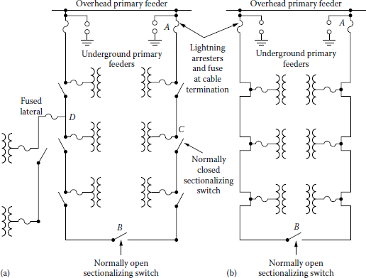
Single-line diagram of loop-type primary-feeder circuits: (a) with a disconnect switch at each transformer and (b) without a disconnect switch at each transformer.
(From Westinghouse Electric Corporation, Electric Utility Engineering Reference Book-Distribution Systems, Vol. 3, East Pittsburgh, Pittsburgh, PA, 1965.)
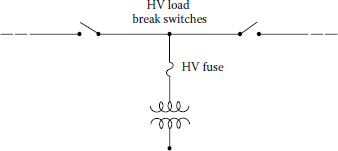
Figure 5.35 shows a distribution transformer with internal high-voltage fuse and with stickoperated plug-in type of high-voltage load-break connectors. Some of the commonly used plug-in types of load-break connector ratings include 8.66 kV line-to-neutral, 200 A continuous 200 A load break, and 10,000 A symmetrical fault close-in rating.
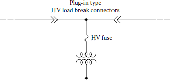
Figure 5.36 shows a distribution transformer with internal high-voltage fuse and with stickoperated high-voltage load-break switches that can be used in Figure 5.34a to allow four modes of operation, namely, the following:
- The transformer is energized and the loop is closed
- The transformer is energized and the loop is open to the right
- The transformer is energized and the loop is open to the left
- The transformer is de-energized and the loop is open
In Figure 5.33, note that, in case of trouble, the open may be located near one of the underground feed points. Therefore, at least in this illustrative design, the single-phase underground cables should be at least ampacity sized for the load of 12 blocks, not merely six blocks.
In Figure 5.33, note further the difficulty in providing abundant overvoltage protection to cable and distribution transformers by placing lightning arresters at the open cable ends. The location of the open moves because of switching, whether for repair purposes or for load balancing.
Example 5.2
Consider the layout of the area and the annual peak demands shown in Figure 5.32. Note that the peak demand per lateral is found as
Assume a lagging-load power factor of 0.90 at all locations in all primary circuits at the time of the annual peak load. For purposes of computing voltage drop in mains and in three-phase laterals, assume that the single-phase load is perfectly balanced among the three phases. Idealize the voltage-drop calculations further by assuming uniformly distributed load along all laterals. Assume nominal operating voltage when computing current from the kilovoltampere load.
For the open-wire overhead copper lines, compute the percent voltage drops, using the precalculated percent voltage drop per kilovoltampere–mile curves given in Chapter 4. Note that Dm = 37 in. is assumed.
The joint EEI-NEMA report [6] defines favorable voltages at the point of utilization, inside the buildings, to be from 110 to 125 V. Here, for illustrative purposes, the lower limit is arbitrarily raised to 116 V at the meter, that is, at the end of the service-drop cable. This allowance may compensate for additional voltage drops, not calculated, due to the following:
- Unbalanced loading in three-wire single-phase secondaries
- Unbalanced loading in four-wire three-phase primaries
- Load growth
- Voltage drops in building wiring
Therefore, the voltage criteria that are to be used in this problem are
and
at the meter. The maximum voltage drop, from the low-voltage bus of the distribution substation to the most remote meter, is 7.50%. It is assumed that a 3.5% maximum steady-state voltage drop in the secondary distribution system is reasonably achievable. Therefore, the maximum allowable primary voltage drop for this problem is limited to 4.0%.
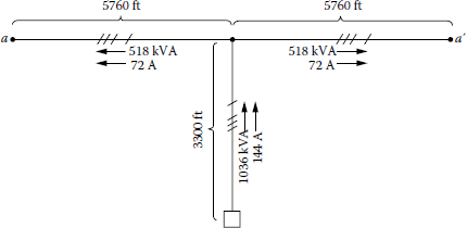
Assume open-wire overhead primaries with three-phase four-wire laterals, and that the nominal voltage is used as the base voltage and is equal to 2400/4160 V for the three-phase fourwire grounded-wye primary system with copper conductors and Dm = 37 in. Consider only the "longest" primary circuit, consisting of a 3300 ft main and the two most remote laterals,* like the laterals a and a' of Figure 5.32. Use ampacity-sized conductors but in no case smaller than AWG #6 for reasons of mechanical strength. Determine the following:
- The percent voltage drops at the ends of the laterals and the main.
- If the 4% maximum voltage-drop criterion is exceeded, find a reasonable combination of larger conductors for main and for lateral that will meet the voltage-drop criterion.
Solution
- Figure 5.37 shows the "longest" primary circuit, consisting of the 3300 ft main and the most remote laterals a and a'. In Figure 5.37, the signs //// indicate that there are three phase and one neutral conductors in that portion of the one-line diagram. The current in the lateral is
Thus, from Table A.1, AWG #6 copper conductor with 130-A ampacity is selected for the laterals. The current in the main is
Hence, from Table A.1, AWG #4 copper conductor with 180-A ampacity is selected for the mains. Here, note that the AWG #5 copper conductors with 150-A ampacity are not selected due to the resultant too-high total voltage drop.
From Figure 4.17, the K constants for the AWG #6 laterals and the AWG #4 mains can be found as 0.015 and 0.01, respectively. Therefore, since the load is assumed to be uniformly distributed along the lateral,
and since the main is considered to have a lumped-sum load of 1036 kVA at the end of its length,
Therefore, the total percent primary voltage drop is
which exceeds the maximum primary voltage-drop criterion of 4.00%.
Here, note that if single-phase laterals were used instead of the three-phase laterals, according to Morrison [7], the percent voltage drop of a single-phase circuit is approximately four times that for a three-phase circuit, assuming the use of the same-size conductors. Hence, for the laterals,
Therefore, from Equation 5.95, the new total percent voltage drop would be
which would be far exceeding the maximum primary voltage-drop criterion of 4.00%.
- Therefore, to meet the maximum primary voltage-drop criterion of 4.00%, from Table A.1, select 4/0 and AWG #1 copper conductors with ampacities of 480 A and 270 A for the main and laterals, respectively. Hence, from Equation 5.93,
and from Equation 5.94,
Therefore, from Equation 5.95,
which meets the maximum primary voltage-drop criterion of 4.00%.
Example 5.3
Repeat Example 5.2 but assume that, instead of the open-wire overhead primary system, a selfsupporting aerial messenger cable with aluminum conductors is being used. This is to be considered one step toward the improvement of the aesthetics of the overhead primary system, since, in general, very few crossarms are required.
Consider again only the "longest" primary circuit, consisting of a 3300 ft main and the two most remote laterals,* like the laterals a and a' of Figure 5.32. For the voltage-drop calculations in the self-supporting aerial messenger cable, use Table A.23 for its resistance and reactance values. For ampacities, use Table 5.2, which gives data for XLPE-insulated aluminum conductor, grounded neutral +3/0 aerial cables. These ampacities are based on 40°C ambient and 90°C conductor temperatures and are taken from the General Electric Company's Publication No. PD-16.
Current-Carrying Capacity of XLPE Aerial Cables
Ampacity, A |
||
|---|---|---|
Conductor Size |
5 kV Cable |
15 kV Cable |
6 AWG |
75 |
|
4 AWG |
99 |
|
2 AWG |
130 |
135 |
1 AWG |
151 |
155 |
1/0 AWG |
174 |
178 |
2/0 AWG |
201 |
205 |
3/0 AWG |
231 |
237 |
4/0 AWG |
268 |
273 |
250 kcmil |
297 |
302 |
350 kcmil |
368 |
372 |
500 kcmil |
459 |
462 |
Solution
- The voltage drop, due to the uniformly distributed load, at the lateral is
where
I = 72 A, from Example 5.2
r = 4.13 Ω/min, for AWG #6 aluminum conductors from Table A.23
xL = 0.258 Ω/min, for AWG #6 aluminum conductors from Table A.23
cos θ = 0.90
sin θ = 0.436
Therefore,
or, in percent,
The voltage drop due to the lumped-sum load at the end of main is where
where
I = 144 A, from Example 5.2
r = 1.29 Ω/min, for AWG #1 aluminum conductors from Table A.23
xL = 0.211 Ω/min, for AWG #1 aluminum conductors from Table A.23
Therefore,
or, in percent,
Thus, from Equation 5.95, the total percent primary voltage drop is
which far exceeds the maximum primary voltage-drop criterion of 4.00%.
- Therefore, to meet the maximum primary voltage-drop criterion of 4.00%, from Tables 5.2 and A.23, select 4/0 and 1/0 aluminum conductors with ampacities of 268 A and 174 A for the main and laterals, respectively.
Hence, from Equation 5.97,
or, in percent,
From Equation 5.98,
or, in percent,
Thus, from Equation 5.95, the total percent primary voltage drop is
which meets the maximum primary voltage-drop criterion of 4.00%.
Example 5.4
Repeat Example 5.2, but assume that the nominal operating voltage is used as the base voltage and is equal to 7,200/12,470 V for the three-phase four-wire grounded-wye primary system with copper conductors. Use Dm = 37 in. although Dm = 53 in. is more realistic for this voltage class. This simplification allows the use of the precalculated percent voltage drop per kilovoltampere–mile curves given in Chapter 4.
Consider serving the total area of 12 × 10 = 120-block area, shown in Figure 5.32, with two feeder mains so that the longest of the two feeders would consist of a 3300 ft main and 10 laterals, that is, the laterals a through e and the laterals a' through e'. Use ampacity-sized conductors, but not smaller than AWG #6, and determine the following:
- Repeat part (a) of Example 5.2.
- Repeat part (b) of Example 5.2.
- The deliberate use of too-small D leads to small errors in what and why?
Solution
- The assumed load on the longer feeder is
Therefore, the current in the main is
Thus, from Table A.1, AWG #2, three-strand copper conductor, is selected for the mains. The current in the lateral is
Hence, from Table A.1, AWG #6 copper conductor is selected for the laterals.
From Figure 4.17, the K constants for the AWG #6 laterals and the AWG #2 mains can be found as 0.00175 and 0.0008, respectively. Therefore, since the load is assumed to be uniformly distributed along the lateral, from Equation 5.93,
and since, due to the peculiarity of this new problem, one-half of the main has to be considered as an express feeder and the other half is connected to a uniformly distributed load of 5180 kVA,
Therefore, from Equation 5.95, the total percent primary voltage drop is
- It meets the maximum primary voltage-drop criterion of 4.00%.
- Since the inductive reactance of the line is
or
when Dm = 37 in.,
and when Dm = 53 in.,
Hence, there is a difference of
which calculates a voltage-drop value smaller than it really is.
Example 5.5
Consider the layout of the area and the annual peak demands shown in Figure 5.33. The primary distribution system in the figure is a mixed system with overhead mains and a URD system. Assume that open-wire overhead mains are used with 7,200/12,470 V three-phase four-wire grounded-wye ACSR conductors and that Dm = 53 in. Also assume that concentric neutral XLPEinsulated underground cable with aluminum conductors is used for single-phase and 7200 V underground cable laterals.
For voltage-drop calculations and ampacity of concentric neutral XLPE-insulated URD cable with aluminum conductors, use Table 5.3.
The foregoing data are for a currently used 15 kV solidly grounded neutral class of cable construction consisting of (1) Al phase conductor, (2) extruded semiconducting conductor shield, (3) 175 mils thickness of cross-linked PE insulation, (4) extruded semiconducting sheath and insulation shield, and (5) bare copper wires spirally applied around the outside to serve as the current-carrying grounded neutral. The data given are for a cable intended for single-phase service, hence the number and the size of concentric neutral are selected to have "100% neutral" ampacity. When three such cables are to be installed to make a three-phase circuit, the number and/or size of copper concentric neutral strands on each cable are reduced to 33% (or less) neutral ampacity per cable.
Another type of insulation in current use is high-molecular-weight PE (HMWPE). It is rated for only 75°C conductor temperature and, therefore, provides a little less ampacity than XLPE insulation on the same conductor size. The HMWPE requires 220 mils insulation thickness in lieu of 175 mil. Cable reactances are, therefore, slightly higher when HMWPE is used. However, the ΔXL is negligible for ordinary purposes.
15 kV Concentric Neutral XLPE-Insulated Al URD Cable
Ω/1000 fta |
Ampacity, A |
||||
|---|---|---|---|---|---|
Al Conductor Size |
Cu Neutral |
rb |
XL |
Direct Burial |
In Duct |
4 AWG |
6-#14 |
0.526 |
0.0345 |
128 |
91 |
2 AWG |
104 14 |
0.331 |
0.0300 |
168 |
119 |
1 AWG |
13-#14 |
0.262 |
0.0290 |
193 |
137 |
1/0 AWG |
16-114 |
0.208 |
0.0275 |
218 |
155 |
2/0 AWG |
134 12 |
0.166 |
0.0260 |
248 |
177 |
3/0 AWG |
16-#12 |
0.132 |
0.0240 |
284 |
201 |
4/0 AWG |
20-#12 |
0.105 |
0.0230 |
324 |
230 |
250 kcmil |
25-112 |
0.089 |
0.0220 |
360 |
257 |
300 kcmil |
18-1110 |
0.074 |
0.0215 |
403 |
291 |
350 kcmil |
204 10 |
0.063 |
0.0210 |
440 |
315 |
Source: Data abstracted from Rome Cable Company, URD Technical Manual, 4th edn.
a For single-phase circuitry.
b At 90°C conductor temperature.
The determination of correct r + jXL values of these relatively new concentric neutral cables is a subject of current concern and research. A portion of the neutral current remains in the bare concentric neutral conductors; the remainder returns to the earth (Carson's equivalent conductor). More detailed information about this matter is available in Refs. [8,9]. Use the given data and determine the following:
- Size each of the overhead mains 1 and 2, of Figure 5.33, with enough ampacity to serve the entire 12 × 10 block area. Size each single-phase lateral URD cable with ampacity for the load of 12 blocks.
- Find the percent voltage drop at the ends of the most remote laterals under normal operation, that is, all laterals open at the center, and both mains are energized.
- Find the percent voltage drop at the most remote lateral under the worst possible emergency operation, that is, one main is outaged, and all laterals are fed full length from the one energized main.
- Is the voltage-drop criterion met for normal operation and for the worst emergency operation?
Solution
- Since under the emergency operation the remaining energized main supplies the doubled number of laterals, the assumed load is
Therefore, the current in the main is
Thus, from Table A.5, 300 kcmil ACSR conductors, with 500 A ampacity, are selected for the mains. Since under the emergency operation, due to doubled load, the current in the lateral is doubled,
Therefore, from Table 5.3, AWG #2 XLPE Al URD cable, with 168 A ampacity, is selected for the laterals.
- Under normal operation, all laterals are open at the center, and both mains are energized. Thus the voltage drop, due to uniformly distributed load, at the main is
or
where
I = 480.2/2 = 240.1 A
r = 0.342 Ω/min for 300-kcmil ACSR conductors from Table A.5
xa = 0.458 Ω/min for 300-kcmil ACSR conductors from Table A.5
xd = 0.1802 Ω/min for Dm = 53 in. from Table A.10
cos θ = 0.90
sin θ = 0.436
Therefore,
or, in percent,
The voltage drop at the lateral, due to the uniformly distributed load, from Equation 5.97 is where
where
I = 144/2 = 72 A
r = 0.331 Ω/1000 ft for AWG #2 XLPE Al URD cable from Table 5.3
xL = 0.0300 ft/1000 ft for AWG #2 XLPE Al URD cable from Table 5.3
Therefore,
or, in percent,
Thus, from Equation 5.95, the total percent primary voltage drop is
- Under the worst possible emergency operation, one main is outaged and all laterals are supplied full length from the remaining energized main. Thus the voltage drop in the main, due to uniformly distributed load, from Equation 5.101 is
or, in percent,
The voltage drop at the lateral, due to uniformly distributed load, from Equation 5.97 is
or, in percent,
Therefore, from Equation 5.95, the total percent primary voltage drop is
- The primary voltage-drop criterion is met for normal operation but is not met for the worst emergency operation.
5.14 Primary System Costs
Based on the 1994 prices, construction of three-phase, overhead, wooden pole crossarm-type feeders of normal large conductor (e.g., 600 kcmil per phase) at about 12.47 kV voltage level costs about $150,000 per mile. However, cost can vary greatly due to variations in labor, filing, and permit costs among utilities, as well as differences in design standards, and very real differences in terrain and geology. The aforementioned feeder would be rated with a thermal capacity of about 15 MVA and a recommended economic peak loading of about 10 MVA peal, depending on losses and other costs. At $150,000 per mile, this provides a cost of $10–$15 per kW-mile. Underground construction of three-phase primary is more expensive, requiring buried ductwork and cable, and usually works out to a range of $30–$50 per kW-mile.
The costs of lateral lines vary between about $5 and $15 per kW-mole overhead. The underground lateral lines cost between $5 and $15 per kW-mile for direct buried cables and $30 and $100 per kW-mile for ducted cables. Costs of other distribution equipment, including regulators, capacitor banks and their switches, sectionalizers, and line switches, vary greatly depending on specifics to each application. In general, the cost of the distribution system will vary between $10 and $30 per kW-mile.
Problems
- 5.1 Repeat Example 5.2, assuming a 30 min annual maximum demand of 4.4 kVA per customer.
- 5.2 Repeat Example 5.3, assuming the nominal operating voltage to be 7,200/12,470 V.
- 5.3 Repeat Example 5.3, assuming a 30 min annual maximum demand of 4.4 kVA per customer for a 12.47 kV system.
- 5.4 Repeat Example 5.4 and find the exact solution by using Dm = 53 in.
- 5.5 Repeat Example 5.5, assuming a lagging-load power factor of 0.80 at all locations.
- 5.6 Assume that a radial express feeder used in rural distribution is connected to a concentrated and static load at the receiving end. Assume that the feeder impedance is 0.15 + j0.30 pu, the sending-end voltage is 1.0 pu, and the constant power load at the receiving end is 1.0 pu with a lagging power factor of 0.85. Use the given data and the exact equations for
, and tan δ given in Section 5.12 and determine the following:
- The values and δ by using the exact equations
- The corresponding values of the and currents
- 5.7 Use the results found in Problem 5.6 and Equation 5.90 and determine the receiving-end voltage
- 5.8 Assume that a three-phase 34.5 kV radial express feeder is used in rural distribution and that the receiving-end voltages at full load and no load are 34.5 and 36.9 kV, respectively. Determine the percent voltage regulation of the feeder.
- 5.9 A three-phase radial express feeder has a line-to-line voltage of 22.9 kV at the receiving end, a total impedance of 5.25 + j10.95 Ω/phase, and a load of 5 MW with a lagging power factor of 0.90. Determine the following:
- The line-to-neutral and line-to-line voltages at the sending end
- The load angle
- 5.10 Use the results of Problem 5.9 and determine the percent voltage regulation of the feeder.
- 5.11 Assume that a wye-connected three-phase load is made up of three impedances of 50∠25° Q each and that the load is supplied by a three-phase four-wire primary express feeder. The balanced line-to-neutral voltages at the receiving end are
Determine the following:
- The phasor currents in each line
- The line-to-line phasor voltages
- The total active and reactive power supplied to the load
- 5.12 Repeat Problem 5.11, if the same three load impedances are connected in a delta connection.
- 5.13 Assume that the service area of a given feeder is increasing as a result of new residential developments. Determine the new load and area that can be served with the same percent voltage drop if the new feeder voltage level is increased to 34.5 kV from the previous voltage level of 12.47 kV.
- 5.14 Assume that the feeder in Problem 5.13 has a length of 2 min and that the new feeder uniform loading has increased to three times the old feeder loading. Determine the new maximum length of the feeder with the same percent voltage drop.
- 5.15 Consider a 12.47 kV three-phase four-wire grounded-wye overhead radial distribution system, similar to the one shown in Figure 5.32. The uniformly distributed area of 12 × 10 = 120 – block area is served by one main located in the middle of the service area. There are 10 laterals (6 blocks each) on each side of the main. The lengths of the main and the laterals are 3300 and 5760 ft, respectively. From Table A.1, arbitrarily select 4/0 copper conductor with 12 strands for the main and AWG # 6 copper conductor for the lateral. The K constants for the main and lateral are 0.0032% and 0.00175% VD per kVA-min, respectively. If the maximum diversified demand per lateral is 518.4 kVA, consider the total service area and determine the following:
- The total load of the main feeder in kVA.
- The amount of current in the main feeder.
- The amount of current in the lateral.
- The percent voltage drop at the end of the lateral.
- The percent voltage drop at the end of the main.
- The total voltage drop for the last lateral. Is it acceptable if the 4% maximum voltagedrop criterion is used?
- 5.16 After solving Problem 5.15, use the results obtained, but assume that the main is made up of 500 kcmil, 19-strand copper conductors with Dm = 37 in. and determine the following:
- The percent voltage drop at the end of the main.
- The total voltage drop to the end of last lateral. Is it acceptable and why?
- 5.17 After solving Problem 5.15, use the results obtained, but assume that the main is made up of 350 kcmil, 12-strand copper conductors with Dm = 37 in. and determine the following:
- The percent voltage drop at the end of the main.
- The total voltage drop to the end of last lateral. Is it acceptable and why?
- 5.18 After solving Problem 5.15, use the results obtained, but assume that the main is made up of 250 kcmil, 12-strand copper conductors with Dm = 37 in. and determine the following:
- The percent voltage drop at the end of the main.
- The total voltage drop to the end of last lateral. Is it acceptable and why?
- 5.19 Resolve Example 5.2 by using MATLAB®. Use the same selected conductors and their parameters.
- 5.20 Resolve Example 5.3 by using MATLAB, assuming the nominal operating voltage to be 7,200/12,470 V. Use the same selected conductors and their parameters.
References
1. Fink, D. G. and H. W. Beaty: Standard Handbook for Electrical Engineers, 11th edn., McGraw-Hill, New York, 1978.
2. Westinghouse Electric Corporation: Electric Utility Engineering Reference Book-Distribution Systems, Vol. 3, East Pittsburgh, Pittsburgh, PA, 1965.
3. Gönen, T. et al.: Development of Advanced Methods for Planning Electric Energy Distribution Systems, US Department of Energy, October 1979. Available from the National Technical Information Service, US Department of Commerce, Springfield, VA.
4. Edison Electric Institute: Underground Systems Reference Book, 2nd edn., New York, 1957.
5. Andrews, F. E.: Residential underground distribution adaptable, Electr. World, December 12, 1955, 107–113.
6. EEI-NEMA: Preferred Voltage Ratings for AC Systems and Equipment, EEI Publication No. R-6, NEMA Publication No. 117, May 1949.
7. Morrison, C.: A linear approach to the problem of planning new feed points into a distribution system, AIEE Trans., pt. III (PAS), December 1963, 819–832.
8. Smith, D. R. and J. V. Barger: Impedance and circulating current calculations_for URD multi-wire concentric neutral circuits, IEEE Trans. Power Appar. Syst., PAS-91(3), May/June 1972, 992–1006.
9. Stone, D. L.: Mathematical analysis of direct buried rural distribution cable impedance, IEEE Trans. Power Appar. Syst., PAS-91(3), May/June 1972, 1015–1022.
10. Gönen, T.: High-temperature superconductors, in McGraw-Hill Encyclopedia of Science and Technology, 7th edn., Vol. 7, 1992, pp. 127–129.
11. Gönen, T. and D. C. You: A comparative analysis of distribution feeder costs, Proceeding of the Southwest Electrical Exposition and IEEE Conference, Houston, TX, January 22–24, 1080.
12. Gönen, T.: Power distribution, Chapter 6, in The Electrical Engineering Handbook, 1st edn., Academic Press, New York, 2005, pp. 749–759.
13. Rome Cable Company, URD Technical Manual, 4th edn., Rome, NY, 1962.
* Note that the whole area is not considered here, but only the last two laterals, for practice.