Chapter 12
Electric Power Quality
Only one thing is certain—that is, nothing is certain,
If this statement is true, it is also false.
Ancient Paradox
12.1 Basic Definitions
Harmonics: Sinusoidal voltages or currents having frequencies that are an integer multiples of the fundamental frequency at which the supply system is designed to operate.
Total harmonic distortion (THD): The ratio of the root-mean-square (rms) of the harmonic content to the rms value of the fundamental quantity, expressed as a percent of the fundamental.
Displacement factor (DPF): The ratio of active power (watts) to apparent power (voltamperes).
True power factor (TPF): The ratio of the active power of the fundamental wave, in watts, to the apparent power of the fundamental wave, in rms voltamperes (including the harmonic components).
Triplen harmonics: A term frequency used to refer to the odd multiples of the third harmonic, which deserve special attention because of their natural tendency to be zero sequence.
Total demand distortion (TDD): The ratio of the rms of the harmonic current to the rms value of the rated or maximum demand fundamental current, expressed as a percent.
Harmonic distortion: Periodic distortion of the sign wave.
Harmonic resonance: A condition in which the power system is resonating near one of the major harmonics being produced by nonlinear elements in the system, hence increasing the harmonic distortion.
Nonlinear load: An electric load that draws current discontinuously or whose impedances varies throughout the cycle of the input ac voltage waveform.
Notch: A switching (or other) disturbance of the normal power voltage waveform, lasting less than a half cycle; which is initially of opposite polarity than the waveform. It includes complete loss of voltage for up to a 0.5 cycle.
Notching: A periodic disturbance caused by normal operation of a power electronic device, when its current is commutated from one phase to another.
K-factor: A factor used to quantify the load impact of electric arc furnaces on the power system.
Swell: An increase to between 1.1 and 1.8 pu in rms voltage or current at the power frequency for durations from 0.5 cycle to 1 min.
Overvoltage: A voltage that has a value at least 10% above the nominal voltage for a period of time greater than 1 min.
Undervoltage: A voltage that has a value at least 10% below the nominal voltage for a period of time greater than 1 min.
Sag: A decrease to between 0.1 and 0.9 pu in rms voltage and current at the power frequency for a duration of 0.5 cycles to 1 min.
Cress factor: A value that is displayed on many power quality monitoring instruments representing the ratio of the crest value of the measured waveform to the rms value of the waveform. For example, the cress factor of a sinusoidal wave is 1.414.
Isolated ground: It originates at an isolated ground-type receptacle or equipment input terminal block and terminates at the point where neutral and ground are bonded at the power source. Its conductor is insulated from the metallic raceway and all ground points throughout its length.
Waveform distortion: A steady-state deviation from an ideal sine wave of power frequency principally characterized by the special content of the deviation.
Voltage fluctuation: A series of voltage changes or a cyclical variation of the voltage envelope.
Voltage magnification: The magnification of capacitor switching oscillatory transient voltage on the primary side by capacitors on the secondary side of a transformer.
Voltage interruption: Disappearance of the supply voltage on one or more phases. It can be momentary, temporary, or sustained.
Recovery voltage: The voltage that occurs across the terminals of a pole of a circuit interrupting device upon interruption of the current.
Oscillatory transient: A sudden and nonpower frequency change in the steady-state condition of voltage or current that includes both positive and negative polarity values.
Noise: An unwanted electric signal with a less than 200 kHz superimposed upon the power system voltage or current in phase conductors or found on neutral conductors or signal lines. It is not a harmonic distortion or transient. It disturbs microcomputers and programmable controllers.
Voltage imbalance (or unbalance): The maximum deviation from the average of the three-phase voltages or currents, divided by the average of the three-phase voltages or currents, expressed in percent.
Impulsive transient: A sudden (nonpower) frequency change in the steady-state condition of the voltage or current that is unidirectional in polarity.
Flicker: Impression of unsteadiness of visual sensation induced by a light stimulus whose luminance or spectral distribution fluctuates with time.
Frequency deviation: An increase or decrease in the power frequency. Its duration varies from a few cycles to several hours.
Momentary interruption: The complete loss of voltage (<0.1 pu) on one or more phase conductors for a period between 30 cycles and 3 s.
Sustained interruption: The complete loss of voltage (<0.1 pu) on one or more phase conductors for a time greater than 1 min.
Phase shift: The displacement in time of one voltage waveform relative to other voltage waveform(s).
Low-side surges: The current surge that appears to be injected into the transformer secondary terminals upon a lighting strike to grounded conductors in the vicinity.
Passive filter: A combination of inductors, capacitors, and resistors designed to eliminate one or more harmonics. The most common variety is simply an inductor in series with a shunt capacitor, which short-circuits the major distorting harmonic component from the system.
Active filter: Any of a number of sophisticated power electronic devices for eliminating harmonic distortion.
12.2 Definition of Electric Power Quality
In general, there is no single definition of the term electric power quality that is acceptable by everyone. According to Heydt [3], the electric power quality can be defined “as the goodness of the electric power quality supply in terms of its voltage wave shape, its current wave shape, its frequency, its voltage regulation, as well as level of impulses, and noise, and the absence of momentary outages.”
Occasionally, some additional considerations are included in the definition of electric power quality. These concerns include reliability, electromagnetic compatibility, and even generation supply concerns. Distribution engineers usually focus on the load bus voltage in terms of maintaining its rated sinusoid voltage and frequency, in addition to other concerns, including spikes, notches, and outages. The growing utilization of electronic equipment has increased the interest in power quality in recent year.
The more specific definitions of the electric power quality depend on the points of view. For example, some utility companies may define power quality as reliability and point out to statistics demonstrating that the power system is 99.98% reliable. The equipment manufacturers may define it as those characteristics of the power supply that enable their equipment to work properly.
However, customers may define the electric power quality in terms of the absence of any power quality problems. From the customer point of view, the power quality problem is defined as “any power problem manifested in voltage, current, or frequency deviations that result in failure or unsatisfactory operation of customer’s equipment” [4].
In general, electric power quality issues cover the entire electric power system, but their main emphases are in the primary and secondary distribution systems. Since usually the loads cause the distortion in bus voltage wave shape and are generally connected to the secondary system, the secondary system receives more attention than the primary system. However, occasionally, transmission and generation system are also included in some power quality analysis and evaluations.
12.3 Classification of Power Quality
The electric power quality disturbances can be classified in terms of the steady-state disturbance that is often periodic and lasts for a long period of time and the transient disturbance that generally lasts for a few milliseconds and then decays down to zero.
The first one is usually less obvious, less harmful, and lasts for a long time, but the cost involved may be very high. The second one is usually more obvious in its harmful effects and the costs involved may be extremely high. In the United States, it is estimated that the annual cost of transient power quality problems is anywhere between 100 million and 3 billion dollars, depending on the year [3].
The electric power quality issues include a wide variety of electromagnetic phenomena on the power systems. The International Electrotechnical Commission (IEC) classifies electromagnetic phenomena into various groups, as given in Table 12.1. Note that the definition of waveform distortion includes harmonics, interharmonics, dc in ac networks, and notching phenomena. The categories and characteristics of power system electromagnetic phenomena are given in Table 12.2.
Classification of Electromagnetic Disturbances according to IEC
Conducted Low-Frequency Phenomena
Radiated Low-Frequency Phenomena
Conducted High-Frequency Phenomena
Radiated High-Frequency Phenomena
Electrostatic Discharge Phenomena (ESD) Nuclear Electromagnetic Pulse (NEMP) |
Categories and Characteristics of Power System Electromagnetic Phenomena
Categories |
Typical Spectral Content |
Typical Duration |
Typical Voltage Magnitude |
|---|---|---|---|
1.0 Transients |
|||
1.1 Impulsive |
|||
• Nanosecond |
5 ns rise |
<50 ns |
|
• Microsecond |
1 μs rise |
50 ns–1 ms |
|
• Millisecond |
0.1 ms rise |
>1 ms |
|
1.2 Oscillatory |
|||
• Low frequency |
<5 kHz |
0.3–50 ms |
0–4 pu |
• Medium frequency |
5–500 kHz |
20 μs |
0–8 pu |
• High frequency |
0.5–5 MHz |
5 μs |
0–4 pu |
2.0 Short-duration variations |
|||
2.1 Instantaneous |
|||
• Interruption |
0.5–30 cycles |
<0.1 pu |
|
• Sag (dip) |
0.5–30 cycles |
0.1–0.9 pu |
|
• Swell |
0.5–30 cycles |
1.1–1.8 pu |
|
2.2 Momentary |
|||
• Interruption |
30 cycles–3 s |
<0.1 pu |
|
• Sag (dip) |
30 cycles–3 s |
0.1–0.9 pu |
|
• Swell |
30 cycles–3 s |
1.1–1.4 pu |
|
2.3 Temporary |
|||
• Interruption |
3 s–1 min |
<0.1 pu |
|
• Sag (dip) |
3 s–1 min |
0.1–0.9 pu |
|
• Swell |
3 s–1 min |
1.1–1.2 pu |
|
3.0 Long-duration variations |
|||
3.1 Interruption, sustained |
>1 min |
0.0 pu |
|
3.2 Undervoltages |
>1 min |
0.8–0.9 pu |
|
3.3 Overvoltages |
>1 min |
1.1–1.2 pu |
|
4.0 Voltage distortion |
Steady state |
0.5%–2% |
|
5.0 Waveform distortion |
|||
5.1 DC offset |
Steady state |
0%–0.1% |
|
5.2 Harmonics |
0–100th harmonic |
Steady state |
0%–20% |
5.3 Interharmonics |
0–6 KHz |
Steady state |
0%–2% |
5.4 Notching |
Steady state |
||
5.5 Noise |
Broadband |
Steady state |
0–1% |
6.0 Voltage fluctuations |
<25 Hz |
Intermittent |
0.1%–7% |
7.0 Power frequency variations |
<10 s |
Note that long-duration voltage variations can be either overvoltages or undervoltages. They generally are not the result of system faults, but are caused by load variations on the system and system switching operations.
A sag, or dip, is a decrease to between 0.1 and 0.9 pu in rms voltage or current at the power frequency for durations from 0.5 cycles to 1 min. A swell is an increase to between 1.1 and 1.8 pu in rms voltage or current at the power frequency for durations from 0.5 cycle to 1 min. As with sags, swells are usually associated with system fault conditions, but they are not a common a voltage sags.
Typical examples of swell-producing events include the temporary voltage rise on the unfaulted phases during an SLG fault. Swells can also be caused by switching off a large load or energizing a large capacitor bank. Waveform distortion is defined as a steady-state deviation from an ideal sine wave.
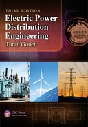
The main types of waveform distortions include dc offset, harmonics, interharmonics, notching, and noise. Figure 12.1 shows various types of disturbances. In the United States, most of residential, commercial, and industrial systems use line-to-neutral voltages that are equal or less than 277 V. The basic sources and characteristics of surges and transients in primary and secondary distribution networks are given in Table 12.3.
Various types of disturbances: (a) harmonic distortion, (b) noise, (c) notches, (d) sag, (e) swell, and (f) surge.
Sources and Characteristics of Surge Voltages in Primary and Secondary Distribution Circuit
Type |
Source |
Characteristics |
|---|---|---|
System switching transients |
Line switching, capacitor switching |
Propagates in secondary circuits with attenuation at distribution transformers |
Minor load switching |
Switching of large commercial or residential loads |
|
Transients resulting from circuit breaker and fuse operations due to faults |
Fast breakers (e.g., vacuum) may cause high-current interruption in the μs range. |
|
Lightning |
Direct stroke to primary |
Worst case can be in 100 kA range. Typical impulse in primary in the range of 1–6 kA. |
Stroke near primary |
Induced in adjacent circuit by magnetic induction. Amplitude of impulse dependent on proximity and intensity of stroke. |
|
Direct stroke to secondary |
Worst case can be in 100 kA range. Typical impulses in 0.5–6 kA range. |
|
Stoke near secondary |
Induced in adjacent circuits by magnetic induction. Overhead circuits with considerable exposure are most likely to experience near-stoke phenomenon (e.g., rural electric circuits). |
|
Common ground current |
Distribution of lightning stokes currents in the earth and in metallic ground circuits cause common coupling with power system ground circuits. |
Source: Heydt, G.T., Electric Power Quality, Ist edn., Stars in a Circle Publications, West LaFayatte, IN, 1991.
12.4 Types of Disturbances
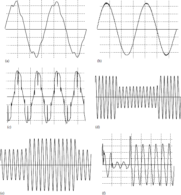
Switching of reactive loads, for example, transformers and capacitors, create transients in the kilohertz range. Figure 12.2a shows phase-neutral transients resulting from addition of capacitive load. Figure 12.2b shows neutral-ground transient resulting from addition of inductive load. Electromechanical switching device interacts with the distributed inductance and capacitance in the ac distribution and loads to create electric fast transients (EFTs). For example, Figure 12.2c shows phase-neutral transients resulting from arching and bouncing contactor.
12.4.1 Harmonic Distortion
Harmonics is blamed for many power quality disturbances that are actually transients. Even though transient disturbances may also have high-frequency components (not associated with the system fundamental frequency), transients and harmonics are distinctly different phenomena and are analyzed differently. Transients are usually dissipated within a few cycles, for example, transients that result from switching a capacitor bank.
In contrast, harmonics take place in steady state and are integer multiples of the fundamental frequency. Also, the waveform distortion that produces the harmonics is continuously present or at least for several seconds. Usually, harmonics are associated with the continuous operation of a load. However, transformer energization is a transient case but can result in a significant waveform distortion for many seconds. Furthermore, this is known to cause system resonance, especially when an underground cabled system is being fed by the transformer.
Harmonic distortion is caused by nonlinear devices in the distribution system. Here, a nonlinear device is defined as the one in which the current is not proportional to the applied voltage, that is, while the applied voltage is perfectly sinusoidal, the resulting current is distorted. Increasing the voltage by a small amount may cause the current to double and take on a different wave shape.
Any periodic and distorted waveform can be expressed as a sum of sinusoids with different frequencies. When the waveform is identical from one cycle to the next, it can be represented by the sum of pure sine waves in which the frequency of each sinusoid is an integer multiple of the fundamental frequency of the distorted wave. This multiple is called a harmonic of the fundamental. The sum of sinusoids is referred to as a Fourier series. In this way, it is much easier to determine the system resonance to an input that is sinusoidal.
For example, the system is analyzed separately at each harmonic using the conventional steadystate analysis techniques. The outputs at each frequency are then combined to form a new Fourier series, from which the output waveform may be determined, if necessary. Usually, only the magnitudes of the harmonics are needed. When both the positive and negative half cycles of a waveform have identical shapes, the Fourier series has only odd harmonics.
The presence of even harmonics is often an indication that there is something wrong either with the load equipment or with the transducer used to make the measurement. However, there are exceptions, for example, half-wave rectifiers and arc furnaces when the arc is random.
In a distribution system, most nonlinearities can be found in its shunt elements, that is, loads. Its series impedance, that is, short-circuit impedance between the sources and the load, is sufficiently nonlinear. Nonlinear loads appear to be sources of harmonic current in shunt with and injecting harmonic currents into the power system. For most of harmonics study, it is customary to treat these harmonic-generating loads simply as harmonic current sources, that is, harmonic current generators.
Harmonics, which do little or no useful work, cause extra power losses in distribution transformers, feeders, and some conventional loads such as motors. Harmonics also cause interference in communication circuits, resonance in power systems, and abnormal operations of protection and control equipment.
In the past, most harmonic problems were caused by large single-phase harmonic sources, and they were handled effectively on a case-by-case basis. However, because of the growing use of harmonic-generating power electronic loads, the background distortion levels are gradually increasing. Dealing with such problems is more difficult than dealing with those caused by single-harmonic sources.
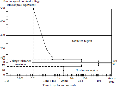
12.4.2 CBEMA and ITI Curves
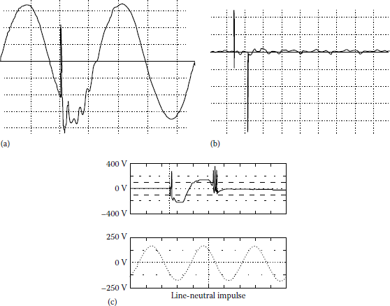
Protection of the equipment against the hostile environment is the goal of the technology of electromagnetic compatibility. The Computer Business Equipment Manufacturer Association (CBEMA) has developed the CBEMA curve, shown in Figure 12.3, which can be used to evaluate the voltage quality of a power system with respect to voltage interruptions, dips or undervoltages, and swells or overvoltages.
It was developed as a guideline to help CBEMA members in the design of the power supply for their computer and electronic equipment. A portion of the curve was adopted IEEE Standard (Std.) 446 that is typically used in the analysis of power quality monitoring results.
The curve shows the magnitude and duration of voltage variations on the power system. The region between the two sides of the curve is the tolerance envelope within which electronic equipment is expected to operate reliably.
In power systems, the only portion of the curve that is used is from 0.1 cycles and higher due to limitations in power quality monitoring instruments. The CBEMA has been replaced by ITI curve, shown in Figure 12.4. It is similar to the CBEMA curve and specifically applies to common 120 V computer equipment. Although developed for 120 V computer equipment, the curve has been applied to general power quality equipment. This curve is also being used in power quality studies.
12.5 Measurements of Electric Power Quality
12.5.1 RMS Voltage and Current
The expressions for the rms voltage and current are
Vrms=∞∑h=1(Vh√2)2(12.1)
and
Irms=∞∑h=1(Ih√2)2(12.2)
Here, it is assumed that Vh and Ih are also given in rms.
12.5.2 Distribution Factors
There are several indices that have been used to measure electric power quality. The most widely used one is the total harmonic distortion (THD). The total harmonic distortion THDV, also known as the voltage distortion factor (VDF), is defined as
THDV=√∑∞h=2V2hV1(12.3a)
or
THDV=√(VrmsV1)2−1(12.3b)
where
- Vh is the harmonic voltage at harmonic frequency “h” in rms
- V1 is the rated fundamental voltage in rms
- h is the harmonic order (h = 1 corresponds to the fundamental)
Similarly, the total harmonic distortion THDI, also known as the current distortion factor (CDF), is defined as
THDI=√∑∞h=2I2hI1(12.4a)
or
THDI=√(IrmsI1)2−1(12.4b)
where
- Ih is the harmonic current at harmonic frequency “h” in rms
- I1is the rated fundamental current in rms
The rms voltage and current can now be expressed in terms of THD as
Vrms=√∞∑h=1V2h=V1√1+THD2V(12.5)
and
Irms=√∞∑h=1I2h=I1√1+THD2I(12.6)
For balanced three-phase voltages, the line-to-line neutral voltage is used in Equation 12.3. But, in the unbalanced case, it is necessary to calculate a different THD for each phase. The voltage THD is almost always a meaningful number. However, this is not the case for the current.
The current THD definition causes some confusion because there is a nonlinear relationship between the magnitude of the harmonic components and percent THD. With the definition of THD, one losses an intuitive feeling for how distorted a particular wave form may be. Distortions greater than 100% are possible, and a waveform with 120% does not contain twice the harmonic components of a waveform with 60% distortion. For the lower levels (less than 10%) of THD, the THD definition is fairly linear. But, for higher levels of THD, which are possible for real-world current distortion, the THD definition is very nonlinear. Also, a small current may have a high THD but not be a significant threat to the system.
This difficulty may be avoided by referring THD to the fundamental of the peak demand current rather than the fundamental of the present sample. This is called total demand distortion (TDD) and serves as the basis for the guidelines in IEEE Std. 519-1992. Therefore,
TDD = √∑∞h=2I2hIL×100(12.7)
where IL is the maximum demand load current in rms amps.
When discussing distortion in power distribution systems, it is important to be specific as to the quantity being measured and the conditions of measurements. For example, an equipment may have an “output distortion of 5%.” Is this voltage or current distortion? Under what load conditions is it taking place? Transformers often have a specification such as “1% maximum output voltage distortion.”
What is not stated is that this voltage distortion specification applies only to a linear load and that the transformer-generated voltage distortion (i.e., 1%) is additive to any voltage distortion that may be present on the input voltage source. When supplying nonlinear loads, the transformer voltage distortion will be higher.
Finally, the distortion index (DIN) is commonly used in countries outside of North America. It is defined as
DIN = √∑∞h=2V2h∑∞h=1V2h(12.8)
from which
DIN = THD√1+THD2(12.9)
12.5.3 Active (Real) and Reactive Power
The following relationships are for active (real) and reactive power apply. Active power is
p(t)=v(t)×i(t)(12.10)
which has the average
P=1TT∫0p(t)dt(12.11a)
or
P=12∞∑h=1vhihcos(θh−ϕh)(12.11b)
or
P=∞∑h=1VhIhcos(θh−ϕh)(12.11c)
The real power is defined as
Q=12∞∑h=1vhihsin(θh−ϕh)(12.12a)
or
Q=∞∑h=1VhIhsin(θh−ϕh)(12.12b)
12.5.4 Apparent Power
Based on the aforementioned formulas for voltage and current, the apparent power is
S=VrmsIrms(12.13a)
or
S=√∞∑h=1V2hI2h(12.13b)
or
S=V1I1√1+THD2V√1+THD2I(12.13c)
or
S=S1√1+THD2V√1+THD2I(12.13d)
where S1 is the apparent power at the fundamental frequency.
12.5.5 Power Factor
For purely sinusoidal voltage and current, the average power (or true average active power)
Pavg=12VmImcosθ(12.14)
or
Pavg=VrmsIrmscosθ(12.15)
where
cos θ is the power factor (PF)
For the sake of simplicity in notation, Equation 12.15 can be expressed as
The cos θ factor is called the PF. It is said that the PF leads when the current leads the voltage and lags when the current lags the voltage:
This PF is now called the displacement power factor (DF). Also,
But, for the nonsinusoidal case,
or
Note that here, the Vh and Ih quantities are the peak quantities:
or
Therefore, because of harmonic distortion,
but
where
or
or
or
Here, D represents distortion power and is called distortion voltamperes. It represents all cross products of voltage and current at different frequencies, which yield no average power. Since the PF is a measure of the power utilization efficiency of the load,
Thus,
or
The PFs that can be found from Equation 12.26a and b are called the true power factor (TPF). The PF that can be found from Equation 12.10 is redefined as the displacement power factor. Also, the TPF can be expressed as
or
where
- DF = P/S1 is the displacement power factor
- DPF is the distortion power factor
or
or
Note that when harmonics are involved, from Equation 12.26, the TPF is
Furthermore, one should not be mislead by a nameplate PF of unity. The unity PF is attainable only with pure sinusoids. What is actually provided is the displacement PF.
Power quality monitoring instruments now commonly report both the displacement factors as well as the TPFs. The displacement factor is typically used in determining PF adjustments on a utility bill since it is related to the displacement of the fundamental voltage and current.
However, sizing capacitors for PF correction is no longer simple. It is not possible to get unity PF due to the distortion power presence. In fact, if resonance effects are significant after installing the capacitors, D can become large and PF would decrease. (In most cases, D is less than 5%.) This results from the fact that the power is proportional to the product of voltage and current.
Capacitors basically compensate only for the fundamental frequency reactive power and cannot completely correct the TPF to unity when there are harmonics present. In fact, capacitors can make the PF worse by creating resonance conditions that magnify the harmonic distortion.
The maximum to which the TPF that can be corrected can approximately be found from
where
- THDI is in per units
- THDV is zero
12.5.6 Current and Voltage Crest Factors
The current crest factor (CCF) is defined as
and the voltage crest factor (VCF) is defined as
Neglecting phase angles, the total peak current or voltage would be
or
The corresponding pu increase in total peak current or voltage is then
or
Note that is only true for the case of a pure sinusoid, and the same applies for voltage.
Example 12.1
Based on the output of a harmonic analyzer, it has been determined that a nonlinear load has a total rms current of 75 A. It also has 38, 21, 4.6, and 3.5 A for the third, fifth, seventh, and ninth harmonic currents, respectively. The instrument used in has been programmed to present the resulting data in amps rather than in percentages. Based on the given information, determine the following:
- The fundamental current in amps
- The amounts of the third, fifth, seventh, and ninth harmonic currents in percentages
- The amount of the THD
Solution
- Since
- Hence,
- Since
Thus,
or
or
12.5.7 Telephone Interference and the I · T Product
Harmonics generate telephone interference through inductive coupling. The I · T product, used to measure telephone interference, is defined as
where Th is the telephone interference weighting factor at the hth harmonic. (It includes the audio effects as well as inductive coupling effects.)
The telephone interference factor (TIF) is defined as
Table 12.4 gives the telephone interference weighting factors for various harmonics based on Table 12.2 of IEEE Std. 519-1992.
Standard Telephone Interference Weighting Factors
h |
1 3 |
5 |
7 |
9 |
11 |
13 |
15 |
17 |
19 |
21 |
23 |
|---|---|---|---|---|---|---|---|---|---|---|---|
Th |
0.5 30 |
225 |
650 |
1320 |
2260 |
3360 |
4350 |
5100 |
5630 |
6050 |
6370 |
Example 12.2
A 4.16 kV three-phase feeder is supplying a purely resistive load of 5400 kVA. It has been determined that there are 175 V of zero-sequence third harmonic and 75 V of negative-sequence fifth harmonic. Determine the following:
- The total voltage distortion.
- Is the THD below the IEEE Std. 51-1992 for the 4.16 kV distribution system?
Solution
-
- From Table 12.5, the THDV limit for 4.16 kV is 5%. Since the THD calculated is 4.58%, it is less than the limit of 5% recommended by IEEE Std. 519-1992 for 4.16 kV distribution systems.
IEEE Std. 519-1992 Limits for Harmonic Voltage Distortion in Percent at PCC
2.3–69 kV |
69–161 kV |
>161 kV |
|
|---|---|---|---|
Maximum individual voltage division |
3.0 |
1.5 |
1.0 |
Total voltage distortion, THDv |
5.0 |
2.5 |
1.5 |
Example 12.3
According to ANSI 368 Std., telephone interference from a 4.16 kV distribution system is unlikely to occur when the I · T index is below 10,000. Consider the load given in Example 12.2 and assume that the TIF weightings for the fundamental, the third, and the fifth harmonics are 0.5, 30, and 225, respectively. Determine the following:
- The I1, I3, and I5 currents in amps.
- The I · T1, I · T2, and I · T5 indices.
- The total I · T index.
- Is the total I · T index is less the ANSI 368 Std. limit?
- The total TIF index.
Solution
-
and the resistance is
The harmonic currents are
- The I · T indices are
- Since 7106.72 < 10,000 limit, it is well below the ANSI Std. limit.
- The total TIF index for this case is
Typical requirements of TIF are between 15 and 50.
12.6 Power in Passive Elements
12.6.1 Power in a Pure Resistance
Real (or active) power dissipated in a resistor is given by
where Rh is the resistance at the hth harmonic.
If the resistance is assumed to be constant, that is, ignoring the skin effect, then
Alternatively, expressed in terms of current,
Note that the aforementioned equations can be reexpressed in pu as
where
- P is the total power loss in the resistance
- P1 is the power loss in the resistance at the fundamental frequency
For a purely resistive element, it can be observed from Equation 12.36 that
12.6.2 Power in a Pure Inductance
Power in a pure inductance can be expressed as
where
f1 is the fundamental frequency.
Thus,
so that
or
12.6.3 Power in a Pure Capacitance
Power in a pure capacitance can be expressed as
The negative sign indicates that the reactive power is delivered to the load:
and
Thus,
Hence,
or
12.7 Harmonic Distortion Limits
IEEE Std. 519-1992 is entitled Recommended Practices and Requirements for Harmonic Control in Electric Power Systems [7]. It gives the recommended practice for electric power system designers to control the harmonic distortion that might otherwise determine electric power quality.
The recommended practice is to be used as a guideline in the design of power system with nonlinear loads. The limits set are for steady-state operation and are recommended for “worse-case” conditions. The underlying philosophy is that the customer should limit harmonic currents and the electric utility should limit harmonic voltages.
It does not specify the highest-order harmonics to be limited. Also, it does not differentiate between single-phase and three-phase systems. Thus, the recommended harmonic limits equally apply to both. It does also address direct current that is not a harmonic.
12.7.1 Voltage Distortion Limits
The current edition of IEEE 519-1992 establishes limits on voltage distortion that a utility may supply a user. This assumes almost unlimited ability for the utility to absorb harmonic currents from user. It is obvious that in order for the utility to meet the voltage distortion limits, some limits must be placed on the amount of harmonic current that users can inject the power system.
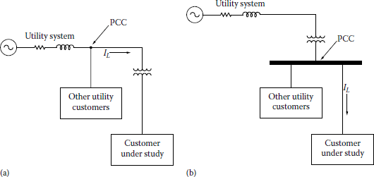
Table 12.5 gives the new IEEE 519 voltage distortion limits at the point of common coupling (PCC) to the utility and other users. The concept of PCC is illustrated in Figure 12.5. It is the location where another customer can be served from the system. It can be located at either the primary or the secondary of a supply transformer depending on whether or not multiple customers are supplied from the transformer.
12.7.2 Current Distortion Limits
The harmonic currents from an individual customer are evaluated at the PCC where the utility can supply other customers. The limits are dependent on the customer load in relation to the system short-circuit capacity at the PCC. Note that all current limits are expressed as a percentage of the customer’s average maximum demand load current.
Table 12.6 gives the new IEEE 519 harmonic current distortion limits at the PCC to the customer. The current distortion limits vary by the size of the user relative to the utility system capacity. The limits attempt to prevent users for a disproportionately using the utility’s harmonic current absorption capacity as well as reducing the possibility of harmonic distortion problems. According to the changes that are suggested in reference [8] include the expansion of voltage levels up to and beyond 161 kV, are included in Tables 12.7 and 12.8, respectively.
IEEE Std. 519-1992 Limits Imposed on Customers (120 V–69 kV) for Harmonic Current Distortion in Percent of IL for Odd Harmonic h at the PCC
ISC/IL |
h < 11 |
11 ≤ h < 17 |
17 ≤ h < 23 |
23 ≤ h < 35 |
35 ≤ h |
TDD |
|---|---|---|---|---|---|---|
4.0 |
2.0 |
1.5 |
0.6 |
0.3 |
5.0 |
|
20–50 |
7.0 |
3.5 |
2.5 |
1.0 |
0.5 |
8.0 |
50–100 |
10.0 |
4.5 |
4.0 |
1.5 |
0.7 |
12.0 |
100–1000 |
12.0 |
5.5 |
5.0 |
2.0 |
1.0 |
15.0 |
>1000 |
15.0 |
7.0 |
6.0 |
2.5 |
1.4 |
20.0 |
a Isc is the short-circuit current at the PCC. IL is the maximum demand load current (fundamental frequency component) also at the PCC. It can be calculated as the average of the maximum monthly demand currents for the previous 12 months or it may have to be estimated.
b All power generation equipment applications are limited to these values of current distortion regardless of the actual short-circuit ratio ISC/IL. The individual harmonic component limits apply to the odd harmonic components. Even harmonic components are limited to 25% of the limits in the table. Current distortions that result in a dc offset, for example, half-wave converters, are not allowed.
IEEE Std. 519-1992 Limits Imposed on Customers (69–161 kV) for Harmonic Current Distortion in Percent of IL for odd Harmonic h at the PCC
ISC/IL |
h < 11 |
11 ≤ h < 17 |
17 ≤ h < 23 |
23 ≤ h < 35 |
35 ≤ h |
TDD |
|---|---|---|---|---|---|---|
<20a |
2.0 |
1.0 |
0.75 |
0.3 |
0.15 |
2.5 |
20–50 |
3.5 |
1.75 |
1.25 |
0.5 |
0.25 |
4.0 |
50–100 |
5.0 |
2.25 |
2.0 |
1.25 |
0.35 |
6.0 |
100–1000 |
6.0 |
2.75 |
2.5 |
1.0 |
0.5 |
7.5 |
>1000 |
7.5 |
3.5 |
3.0 |
1.25 |
0.7 |
10.0 |
a See the footnotes of Table 12.6.
IEEE Std. 519-1992 Limits Imposed on Customers (above 161 kV) for Harmonic Current Distortion in Percent of IL for Odd Harmonic h at the PCC
ISC/IL |
h < 11 |
11 ≤ h < 17 |
17 ≤ h < 23 |
23 ≤ h < 35 |
35 ≤ h |
TDD |
|---|---|---|---|---|---|---|
<50a |
2.0 |
1.0 |
0.75 |
0.3 |
0.15 |
2.5 |
≥50 |
3.5 |
1.75 |
1.25 |
0.5 |
0.25 |
4.0 |
a See the footnotes of Table 12.6.
Since harmonic effects differ substantially depending on the equipment affected, the severity of the harmonic effects imposed on all types of equipment cannot completely be connected to a few simple harmonic indices. Also, the harmonic characteristics of the utility circuit seen from the PCC are often not known accurately. Therefore, good engineering judgment often dictated to review a case-by-case basis. However, through a judicious application of the recommended practice, the interferences between different loads and the system can be minimized. According to IEEE 519-1992, the evaluation procedure for newly installed nonlinear loads includes the following:
- Definition of the PCC
- Determination of the Isc, IL, and Isc/IL at the PCC
- Finding the harmonic current and current distortion of the nonlinear load
- Determination of whether or not the harmonic current and current distortions in step 3 satisfy IEEE 519-1992 recommendation limits
- Taking necessary remedies to meet the guidelines
Preventive solutions, such as IEEE 519-1992 guidelines for dealing with harmonics, are the best course of action. However, if these guidelines are not satisfied, the remedial solution, such as passive or active filtering, should be included at the time of installation to avoid potential problems. Meanwhile, the Isc/IL ratio may vary due to different PCC choices. The risk should be reevaluated whenever the Isc/IL ratio is unchanged.
Harmonic controls can be exercised at the utility and end-user sides. IEEE Std.519 attempts to establish reasonable harmonic goals for electric systems that contain nonlinear loads. The objectives are the following: (1) customers should limit harmonic currents, since they have control over their loads; (2) electric utilities should limit harmonic voltages, since they have control over the system impedances; and (3) both parties share the responsibility for holding harmonic levels in check.
12.8 Effects of Harmonics
Harmonics adversely affect virtually every component in the power system with additional dielectric, thermal, and/or mechanical stresses. Harmonics cause increased losses and equipment loss of life. For example, when magnetic devices, such as motors, transformers, and relay coils, are operated from a distorted voltage source, they experience increased heating due to higher iron and copper losses.
Harmonics typically also cause additional audible noise. In motors and generators, severe harmonic distortion can also cause oscillating torques that may excite mechanical resonances. In general, unless specifically designed to accommodate harmonics, magnetic devices should not be operated from voltage sources having more than 5% THD.
Wiring is also affected by harmonic currents. In the case of parallel resonance, the associated wiring may be subjected to abnormally high harmonic current flow. The conductors also experience additional heating beyond the normal I2Rdc losses, due to skin effect and proximity effect that vary by frequency and wiring construction. The ac resistance that includes these effects needs to be calculated at each harmonic current frequency and the wiring ampacity must be derated. Normally, the derating required for harmonic is minimal and can be ignored if conservative wire sizing methods are used.
In general, when capacitors are applied to a power system having significant nonlinear loads, some necessary precautions must be taken to prevent parallel resonance. Even without resonance, additional harmonic current will flow in the capacitors causing additional losses and reduced life. With resonance, the high harmonic voltages and currents can cause capacitor fuses or capacitor failures.
Metering and overcurrent protection can also be affected by harmonics unless they are designed with true-rms sensing. Many devices such as meters and overcurrent protection can be peak or average sensing devices that are rms calibrated assuming sinusoidal waveforms. When nonsinusoidal waveforms are present, significant sensing errors can result. PF meters that are based on phase angle measurements cannot be relied upon with nonlinear loads. Solid state circuit breakers without true-rms sensing may experience nuisance tripping or, worse yet, fail to trip when used with nonlinear loads. Table 12.9 shows various sensing errors under different sensing techniques for various waveforms.
Comparison of Sensing Techniques for Various Waveforms
Average Sensing |
Peak Sensing |
True-RMS |
|
|---|---|---|---|
Waveform |
RMS Calibrated (A) |
RMS Calibrated (A) |
Sensing (A) |
Sine wave |
100 |
100 |
100 |
Square wave |
111 |
71 |
100 |
Triangle wave |
97 |
122 |
100 |
Rectifier-capacitor |
|||
power supply current |
50 |
201 |
100 |
Personal computer load |
833 |
168 |
100 |
Other loads may also be affected by harmonics. The voltage and/or current harmonics can be coupled into sensitive loads and appears as noise or interference, causing degradation of performance or misoperation. Examples of these are voltage harmonics causing picture quality problems in television monitors and current harmonics causing interference in telephone circuits. Some computer systems are also known to be sensitive to voltage distortion, as evidenced by computer vendor specifications that include limits on voltage distortion, typically 5% THD.
Furthermore, harmonics may affect capacitor banks in many ways that include the following:
- Capacitors can be overloaded by harmonic currents. This is due to the fact that their reactances decrease with frequency makes them the sinks for harmonics.
- Harmonics tend to increase the dielectric losses of capacitors, causing additional heating and loss of life.
- Capacitors combined with source inductance may develop a parallel resonant circuits, causing harmonics to be amplified. The resulting voltages may greatly over exceed the voltage ratings of the capacitors, causing capacitor damage and/or blown out fuses. For a remedy, relocating capacitors changes the source-to-capacitor inductive reactance hence prevents the occurrence of the parallel resonance with the supply. Also, varying the reactive power output of a capacitor bank will change the resonant frequency.
12.9 Sources of Harmonics
As explained in Section 8.10, voltage sources, that is, generators, inverters, and transformers, produce voltage distortion. Good generators produce minimal voltage distortions that are usually less than 0.5% THD. Inverter voltage distortion depends on the inverter design.
Most online uninterruptible power supply (UPS) inverters produce less than 4%–5% THD with linear load. Many off-line, that is, standby, UPS inverters produce distorted voltages with greater than 25% of THD.
Transformers add voltage distortion to the input voltage waveform. Most good power transformers will add less than 0.5%–1.0% THD with linear loads.
Today, the major sources of distortion in a power system are the harmonic currents of nonlinear loads. The magnetizing currents of transformers and other magnetic devices are usually quite insignificant. Arc or discharge loads, such as arc furnaces or gas discharge lighting, represent very nonlinear loads. Static power converters represent one of the more widely used nonlinear loads. Static power converters include motor drives, battery charges, UPS, and omnipresent electronic power supply. The levels of current distortion of static power converters are dependent upon their designs. For example, electric power supplies have been observed to produce up to 140% current distortion, while newer designs can have as low as 3% THD.
Succinctly put, harmonic distortion has many causes. Distortion voltage sources will cause harmonic currents to flow in linear loads. Nonlinear loads will draw distorted currents from otherwise sinusoidal voltage source. Distorted currents flowing through the power system impedance will cause voltage distortion.
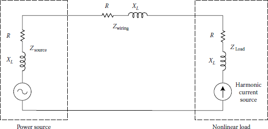
In power systems, the nonlinear load can be modeled as a load for the fundamental current and as a current source for the harmonic currents. The harmonic currents flow from the nonlinear load toward the power source, following the paths of least impedance, as shown in Figure 12.6. The voltage drops in the power system components at each harmonic current frequency will add to, or subtract from, the generated voltage to produce the distorted voltage system.
On radial primary feeders and industrial plant power systems, generally, the harmonic currents flow from the harmonic-producing load toward the power system source, as illustrated in Figure 12.7a. This tendency can be used to locate sources of harmonics. For example, one can use a power quality monitoring device, which is capable of showing harmonic contents of the current, and measure the harmonic currents in each branch, starting at the beginning of the circuit, and trace the harmonics to the source.
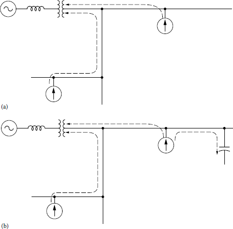
General flow of harmonic currents in a radial power system: (a) without power capacitors and (b) with power capacitors.
However, if there are PF capacitors, this flow pattern can be altered for at least one of the harmonics. For example, adding a capacitor may draw a large amount of harmonic current into that portion of the circuit, as illustrated in Figure 12.7b. Because of this, it is usually required that all capacitors are temporarily disconnected to accurately locate the sources of harmonics.
In the presence of resonance involving a capacitor bank, it is very easy to differentiate harmonic currents due to actual harmonic sources from harmonic currents that are strictly due to resonance. The resonance currents have one dominant harmonic riding on top of the fundamental sinusoidal sine wave. Thus, a large single harmonic almost always indicates resonance.
12.10 Derating Transformers
Transformers serving nonlinear loads exhibit increased eddy current losses due to harmonic currents generated by those loads. Because of this, the transformer rating is derated using a K-factor.
12.10.1 K-Factor
Both the Underwriters Laboratories (UL) and transformer manufacturers established a rating method called K-factor to indicate their suitability for nonsinusoidal load currents.
This K-factor relates transformer capability to serve varying degrees of nonlinear load without exceeding the rated temperature rise limits. It is based on the predicted losses of a transformer. In per unit, the K-factor is
where Ih is the rms current at harmonic h, in per unit of rated rms load current
According to UL specification, the rms current of any single harmonic that is greater than the 10th harmonic be considered as no greater than 1/h of the fundamental rms current.
Today, manufacturers build special K-factor transformers. Standard K-factor ratings are 4, 9, 13, 20, 30, 40, and 50. For linear loads, the K-factor is always one. For nonlinear loads, if harmonic currents are known, the K-factor is calculated and compared against the transformer’s nameplate K-factor. As long as the load K-factor is equal to, or less than, the transformer K-factor, the transformer does not need to be derated.
12.10.2 Transformer Derating
For transformers, ANSI/IEEE Std. C75.110 [5] provides a method to derate the transformer capacity when supplying nonlinear loads. The transformer derating is based on additional eddy current losses due to the harmonic current and that these losses are proportional to the square of the frequency. Thus,
or
where
- Pec-r is the maximum transformer per unit eddy current loss factor (typically, between 0.05 and 0. 10 per units for dry-type transformers)
- Ih is the harmonic current, normalized by dividing it by the fundamental current
- h is the harmonic order
Table 12.10 gives some of the typical values of Pec-r based on the transformer type and size.
Typical Values of Pec-r
Type |
MVA |
Voltage |
Pec-r (%) |
|---|---|---|---|
Dry |
≤1 |
— |
3.8 |
≥1.5 |
5 kV (HV) |
12–20 |
|
≤1.5 |
15 kV (HV) |
9–15 |
|
Oil filled |
≤2.5 |
480 V (LV) |
1 |
2.5–5 |
480 V (LV) |
1–5 |
|
>5 |
480 V (LV) |
9–15 |
Example 12.4
Assume that the per unit harmonic currents are 1.000, 0.016, 0.261, 0.050, 0.003, 0.089, 0.031, 0.002, 0.048, 0.026, 0.001, 0.033, and 0.021 pu A for the harmonic order of 1, 3, 5, 7, 9, 11, 13, 15, 17, 19, 21, 23, and 25, respectively. Also assume that the eddy current loss factor is 8%. Based on ANSI/IEEE Std. C75.110, determine the following:
- The K-factor of the transformer
- The transformer derating based on the standard
Solution
- The results are given in Table 12.11.
Thus, the K-factor is
- According to the standard, the transformer derating is
The Results of Example 12.4, Part (a)
Harmonic (h) |
Currents (pu) |
I2 |
I2 × h2 |
|---|---|---|---|
1 |
1.000 |
1.000 |
1.000 |
3 |
0.016 |
0.000 |
0.002 |
5 |
0.261 |
0.068 |
1.703 |
7 |
0.050 |
0.003 |
0.123 |
9 |
0.003 |
0.000 |
0.001 |
11 |
0.089 |
0.008 |
0.958 |
13 |
0.031 |
0.001 |
0.162 |
15 |
0.002 |
0.000 |
0.001 |
17 |
0.048 |
0.002 |
0.666 |
19 |
0.026 |
0.001 |
0.244 |
21 |
0.001 |
0.000 |
0.000 |
23 |
0.033 |
0.001 |
0.576 |
25 |
0.021 |
0.000 |
0.276 |
Totals |
1.084 |
5.712 |
12.11 Neutral Conductor Overloading
When single-phase electronic loads are supplied with a three-phase four-wire circuit, there is a concern for the current magnitudes in the neutral conductor. Neutral current loading in the three-phase circuits with linear loads is simply a function of the load balance among the three phases. With relatively balanced circuits, the neutral current magnitude is quite small.
In the past, this has resulted in a practice of undersizing the neutral conductor in a relation to the phase conductors. Power system engineers are accustomed to the traditional rule that balanced three-phase systems have no neutral currents. However, this rule is not true when power electronic loads are present.
With electronic loads supplied by switch-made power supplies and fluorescent lighting with electronic ballasts, the harmonic components in the load currents can result in much higher neutral current magnitudes. This is because the odd triplen harmonics (3, 9, 15, etc.) produced by these loads show up as zero-sequence components for balanced circuits.
Instead of canceling in the neutral (as is the case with positive- and negative-sequence components), zero-sequence components add directly in the neutral. The third harmonic is usually the largest singleharmonic component in single-phase power supplies or electronic ballasts. As shown in the next example, the neutral current in such cases will approximately be 173% of the rms phase current magnitude.
The conclusion from this calculation is that neutral conductors in circuits supplying electronic loads should not be undersized. In fact, they should have almost twice the ampacity of the phase conductors. An alternative method to wire these circuits is to provide a neutral conductor with each phase conductor.
Also, many PCs have third harmonic currents greater than 80%. In such cases, the neutral current will be at least 3(80%) = 240% of the fundamental phase current. Therefore, when PC loads dominate a building circuit, it is good engineering practice for each phase to have its own neutral wire or for the shared neutral wire to have at least twice the current rating of each phase wire. Overloaded neutral current are usually only a local problem inside a building, for example, at a service panel.
However, the neutral current concern is not as significant on the 480 V system. The zero-sequence components from the power supply loads are trapped in the delta winding of the step-down transformers to the 120 V circuits. Therefore, the only circuits with any neutral current concern are those supplying fluorescent lighting loads connected to line to neutral, that is, 277 V. In this case, the third harmonic components are much lower.
Typical electronic ballast should not have a third harmonic component exceeding 30% of the fundamental. This means that the neutral current magnitude should always be less than the phase current magnitude in circuits supplying fluorescent lighting load. In these circuits, it is sufficient to make the sizes of neutral conductors the same as the phase conductors.
Office areas and computer rooms with high concentrations of single-phase line-to-neutral power supplies are particularly vulnerable to overheated neutral conductors and distribution transformers. Trends in computer systems over the last several years have increased the likelihood of high neutral currents. Computer systems have shifted from three-phase to single-phase power supplies. Development of switched-mode power supplies allows connection directly to the line-to-neutral voltage without a step-down transformer.
Additionally, there were of buildings not specifically designed to accommodate computer systems. The CBEMA has recognized this concern and alerted the industry to problems caused by harmonics from computer power supplies.
The possible solutions to neutral conductor overloading include the following:
- A separate neutral conductor is provided with each phase conductor in a three-phase circuit that serves single-phase nonlinear loads.
- When a shared neutral is used in a three-phase circuit with single-phase nonlinear loads, the neutral conductor capacity should approximately double the phase-conductor capacity.
- In order to limit the neutral currents, delta–wye transformers specifically designed for nonlinear loads can be used. They should be located as close as possible to the nonlinear loads, for example, computer rooms, to minimize neutral conductor length and cancel triplen harmonics.
- The transformer can be derated, or oversized, in accordance with ANSI/IEEE C57.110 to compensate for the additional losses due to the harmonics.
- The transformers should be provided with supplemental transformer overcurrent protection, for example, winding temperature sensors.
- The third harmonic currents can be controlled by placing filters at the individual loads, if rewiring is an expensive solution.
Example 12.5
In an office building, measurement of a line current of branch circuit serving exclusively computer load has been made using a harmonic analyzer. The outputs of the harmonic analyzer are phase current waveform and the spectrum of current supplying such electronic power loads. For a 60 Hz, 58.5 A rms fundamental current, it is observed from the spectrum that there is 100% fundamental and odd triplen harmonics of 63.3%, 4.4%, 1.9%, 0.6%, 0.2%, and 0.2% for 3rd, 9th, 15th, 21st, 27th, and 33rd order, respectively. If it is assumed that loads on the three phases are balanced and all have this same characteristic, determine the following:
- The approximate rms value of the phase current in per units
- The approximate rms value of the neutral current in per units
- The ratio of the neutral current to the phase current
Solution
- The approximate rms value of the phase current is
where
- The approximate rms value of the neutral current is
- Hence, the ratio of the neutral current to the phase current is
or
Example 12.6
A commercial building is being served by 480 V so that its fluorescent lighting loads can be supplied by a line-to-neutral voltage of 277 V. It is observed that the third harmonic components are much lower. For instance, typical electronic ballast used with the fluorescent lighting should not have a third harmonic component exceeding 30% of the fundamental. For this worse-case analysis, determine the following:
- The approximate rms value of the phase current in per units
- The approximate rms value of the neutral current in per units
- The ratio of the neutral current to the phase current
Solution
- The approximate rms value of the phase current is
- The approximate rms value of the neutral current is
- Hence, the ratio of the neutral current to the phase current is
or
This means that the neutral current magnitude should always be less than the phase current magnitude.
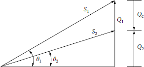
12.12 Capacitor Banks and Power Factor Correction
As discussed in Chapter 8, capacitor banks used in parallel with an inductive load provide this load with reactive power. They reduce the system’s reactive and apparent power and, therefore, cause its PF to increase.
Furthermore, capacitor current causes voltage rise that results in lower line losses and voltage drops loading to an improved efficiency and voltage regulation. Based on the power triangle shown in Figure 12.8, the reactive power delivered by the capacitor bank Qc is
where
- P is the real power delivered by the system and absorbed by the load
- Q1 is the load’s reactive power
- Q2 is the system reactive power after the capacitor bank connection
As it can be observed from the following equation, since a low PF means a high current,
the disadvantages of a low PF include the following: (1) increased line losses, (2) increased generator and transformer ratings, and (3) extra regulation equipment for the case of low lagging PF.
12.13 Short-Circuit Capacity or MVA
Where a new circuit to be added to an existing bus in a complex power system, short-circuit capacity or MVA (or kVA) data provide the equivalent impedance of the power system up to that bus. The three-phase short-circuit MVA is determined from
where
- I3ϕ is the total three-phase fault current in A
- kVL–L is the system phase-to-phase voltage in kV
Alternatively,
from which
It is often in power systems, the short-circuit impedance is equal to the short-circuit reactance, ignoring the resistance and shunt capacitance involved. Hence, the three-phase short-circuit MVA is found from
from which
12.14 System Response Characteristics
All circuits containing both capacitance and inductance have one or more natural resonant frequencies. When one of these frequencies corresponds to an exciting frequency being produced by nonlinear loads, harmonic resonance can occur. Voltage and current will be dominated by the resonant frequency and can be highly distorted. The response of the power system at each harmonic frequency determines the true impact of the nonlinear load on harmonic voltage distortion.
Somewhat surprisingly, power systems are quite tolerant of the currents injected by harmonicproducing loads unless there is some adverse interaction with the system impedance. The response of the power system at each harmonic frequency determines the true impact of the nonlinear load on harmonic voltage distortion.
12.14.1 System Impedance
Since at the fundamental frequency power systems are mainly inductive, their equivalent impedances are also called the short-circuit reactance. In utility distribution systems as well as industrial power systems, capacitive effects are frequently ignored.
The short-circuit impedance Zsc (to the point on a power network at which a capacitor located) can be calculated from fault study results as
where
- Rsc is the short-circuit resistance
- Xsc is the short-circuit reactance
- kVL–L is the phase-to-phase voltage, kV
- MVASC(3ϕ) is the three-phase short-circuit MVA
The inductive reactance portion of the impedance changes linearly with frequency. The reactance at the hth harmonic is found from the fundamental-impedance reactance X1 by
In general, the resistance of most power system components does not change significantly for the harmonics less than the ninth. However, this is not the case for the lines and cables as well as transformers.
For the lines and cables, the resistance changes roughly by the square root of the frequency once the skin effect becomes significant in the conductor at a higher frequency.
For larger transformers, their resistances may vary almost proportionately with the frequency because of the eddy current losses. At utilization voltages, such as industrial power systems, using the transformer impedance XT as Xsc may be a good approximation so that
Generally, this Xsc is about 90% of the total impedance. It usually suffices for the assessment of whether or not there will be a harmonic resonance problem. If the transformer impedance is given in percent, from its per unit value, its impedance value in ohms can be found from
Here, it is assumed that the transformer’s resistance is negligibly small.
12.14.2 Capacitor Impedance
Shunt capacitors substantially change the system impedance variation with frequency. They do not create harmonics. However, severe harmonic distortion can sometimes be attributed to their presence. While the reactance of inductive components increases proportionately to frequency, capacitive reactance Xc decreases proportionately:
where C is the capacitance in farads.
The equivalent line-to-neutral capacitive reactance at the fundamental frequency of a capacitor bank is found from
or
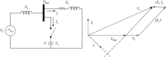
12.15 Bus Voltage Rise and Resonance
Assume that a switched capacitor bank is connected to a bus that has an impedance load, as shown in Figure 12.9, and that the short-circuit capacity of the bus is MVAsc. With the resistance ignored, after the switch is closed, the equivalent (short-circuit) impedance of the system (or the source) is
or in per units,
or
where SB is in MVA and kVB = kVrated.
Also,
or
and the resonant frequency of the system is
or
Since at the resonance,
or
Before the connection of the capacitor bank,
and after the capacitor bank is switched,
where
Assuming that remains constant, the phase voltage rise at the bus due to the capacitor bank connection is
or
Thus,
or
so that
Since
or
or
From Equation 12.74, one can observe that a 0.04 per unit rise in bus voltage due to the switching on a capacitor bank results in a resonance at
Similarly, a 0.02 pu bus voltage rise results in
It can also be shown that
Example 12.7
A three-phase 12.47 kV, 5 MVA capacitor bank is causing a bus voltage increase of 500 V when switched on. Determine the following:
- The per unit increase in bus voltage
- The resonant harmonic order
- The harmonic frequency at the resonance
Solution
- The per unit increase in bus voltage is
- The resonant harmonic order is
- The harmonic frequency at the resonance is